自然语言处理-语言模型的演进与技术剖析

第一章 语言模型介绍

语言模型可以理解为对一句话是否符合正常人表达习惯的一种判断工具。

统计语言模型是所有自然语言处理任务的根基，在语音识别、机器翻译、文本分割、词性标注和信息检索等领域都有广泛应用。传统的统计语言模型是对语言基本单位（通常为句子）的概率分布情况的体现，这一概率分布也是该语言的生成模式。

通俗地说，如果有一句话没有在语料库中出现，我们可以仿照其生成的方式，估算出这句话在语料库中的概率值。一般来说，语言模型可以用各个词语之间条件概率的形式来展现：

$$ p(w*1^n)=p(w_1,w_2,...,w_n)=\prod*{i=1}^np(w_i|Context) $$

其中，$Context$ 为 $w_i$ 的上下文表示。根据 $Context$ 的表示差异，统计语言模型又可以分为不同的类别，其中最具代表性的有$n-gram$语言模型及$nn$语言模型：

第二章 N-gram

$N-gram$ 在自然语言处理（NLP）中是一个极为重要的概念。在 NLP 领域，人们往往基于特定的语料库，借助 $N-gram$ 来实现以下多种功能：

1. 对一个句子是否合理进行预测或评估；
2. 衡量两个字符串之间的差异程度，这也是模糊匹配中常用的方法；
3. 用于语音识别；
4. 应用于机器翻译；
5. 进行文本分类等。

第一节 概率模型

统计语言模型实际上是一个概率模型，所以常见的概率模型都可以用于求解这些参数，参见的概率模型有：N-gram模型、决策树、最大熵模型、隐马尔可夫模型（HMM）、条件随机场（CRT）、神经网络等。

目前常用于语言模型的是$N-gram$模型和神经语言模型：

$$ \begin{aligned} p(S)&=p(w*1,w_2,w_3,w_4,w_5,...,w_n) \\&=p(w_1) \cdot p(w_2|w_1) \cdot p(w_3|w_1,w_2)...p(w_n,w_1,w_2,...,w*{n-1}) \end{aligned} $$

在这个表达式中，$p(S)$表示事件$S$发生的概率。它表示由一系列单词$w_1,w_2,w_3,\cdots,w_n$组成的序列$S$的概率。

假设现在有一句话：我 今天 上午 坐 巴士 去 游乐园。那么从左到右，该句子是有一个顺序的，如下表：

词	概率
我	$p(w_1)$
今天	$p(w_2|w_1)$
上午	$p(w_3|w_1,w_2)$
坐	$p(w_4|w_1,w_2,w_3)$
巴士	$p(w_5|w_1,w_2,w_3,w_4)$
去	$p(w_6|w_1,w_2,w_3,w_4,w_5)$
游乐园	$p(w_7|w_1,w_2,w_3,w_4,w_5, w_6)$

第一个词：“我”出现的概率是$p(w_1)$

第二个词：“今天”是跟在这个“我”后面出现的，那这个时候，就可以认为是$w_2$的出现实际上是以$w_1$作为条件来出现的，那么就可以求得一个条件概率$p(w_2|w_1)$。

第三个词：“上午”是跟在“我”、“今天”后面，“上午”这个词是以前面两个词为条件出现的，那么就可以求得一个条件概率$p(w_3|w_1,w_2)$

……

第 $n$ 个词：它就会以第 $1$ 个词到第 $n-1$ 个词的为条件求得一个概率$p(w_n|w_1,w_2,...,w_{n-1})$

$p(S)$被称为语言模型，即用来计算一个句子概率的模型。

条件概率公式：

$$ \begin{aligned} P(AB)&=P(A|B) \cdot P(B)\\ \end{aligned} $$

事件 A 和事件 B 同时发生的概率 等于 在事件 B 发生的条件下事件 A 发生的概率 乘以 事件 B 发生的概率。

$$ \begin{aligned} P(A|B)&=\frac{P(AB)}{P(B)} \end{aligned} $$

实际上，也可以反过来说 在事件 B 发生的条件下事件 A 发生的概率，等于 事件 A 和事件 B 同时发生的概率 除以 事件 B 发生的概率。

$$ \begin{aligned} p(w*i|w_1,w_2,...,w*{i-1})&=\frac{p(w*1,w_2,...,w*{i-1},w*i)}{p(w_1,w_2,...,w*{i-1})} \end{aligned} $$

由于要计算$w_i$出现的概率，就要去统计前$i-1$词出现的情况，假设词库中有$n$个词，就有$n^{(i-1)}$种可能，这样每增加一个单词，模型的计算成本都指数倍的增长。

分子 $p(w_1,w_2,...,w_{i-1},w_i)$ 是前 $i-1$ 个词和 $w_i$ 同时出现的概率，分母 $p(w_1,w_2,...,w_{i-1})$ 是前 $i-1$ 个词出现的概率。随着词汇数量 $n$ 和词的序列长度 $i$ 的增加，可能的情况数会呈指数级增长，产生两大问题：

• 导致数据变得非常稀疏
• 模型的参数空间也会变得非常大

注意：语料库和词库是不同的概念。

名称	解释
语料库	大量文本的集合，它包含了丰富的语言信息，可以用于语言研究、自然语言处理等领域，通常是一个较大规模的文本集合，其中包含了各种类型的长文本，如文章、书籍、新闻报道等。
词 库	主要是词汇的集合，是对词汇的一种整理和归类，词库更像一本词典。

第二节 马尔科夫假设

马尔科夫假设（Markov Assumption）是指在一个随机过程中，系统在某一时刻的状态仅依赖于其前一个时刻的状态，而与更早的状态无关。

基于马尔科夫假设，$N-gram$语言模型认为一个词出现的概率只与它前面的$n-1$个词相关，假设下一个词的出现依赖它前面的一个词：

$$ \begin{aligned} p(S)&=p(w*1,w_2,w_3,w_4,w_5,...,w_n) \\&=p(w_1) \cdot p(w_2|w_1) \cdot p(w_3|w_1,w_2) ... p(w_n|w_1,w_2,...,w*{n-1}) \\&=p(w*1) \cdot p(w_2|w_1) \cdot p(w_3|w_2) ... p(w_n|w*{n-1}) \end{aligned} $$

第三节 大数定律

大数定律是指在随机现象的大量重复出现中，往往呈现几乎必然的规律。

具体来说，当试验次数足够多时，频率会逐渐接近概率，平均值等统计量也会趋近于相应的数学期望。这一定律在概率论和统计学中具有重要意义。

$$ \begin{aligned} p(w*k|w*{k-1})&=\frac{p(w*{k-1},w_k)}{p(w*{k-1})} \\&\approx\frac{count(w*{k-1}, w_k)}{count(w*{k-1})} \end{aligned} $$

假设下一个词的出现依赖它前面的两个词：

$$ \begin{aligned} p(S)&=p(w*1,w_2,w_3,w_4,w_5,...,w_n) \\&=p(w_1) \cdot p(w_2|w_1) \cdot p(w_3|w_1,w_2) ... p(w_n|w_1,w_2,...,w*{n-1}) \\&=p(w*1) \cdot p(w_2|w_1) \cdot p(w_3|w_1, w_2) ... p(w_n|w*{n-1},w\_{n-2}) \end{aligned} $$

通常情况下，我们管这样的叫$n-gram$模型。

当$N=1$的时候，为一元模型(Unigram model)：

$$ \begin{aligned} p(S)&=p(w_1,w_2,w_3,...,w_n) \\&=p(w_1) \cdot p(w_2) .... p(w_n) \end{aligned} $$

当$N=2$的时候，叫二元模型(Bigram model):

$$ \begin{aligned} p(S)&=p(w*1,w_2,w_3,...,w_n) \\&=p(w_1|start) \cdot p(w_2|w_1) .... p(w_n|w*{n-1}) \end{aligned} $$

当$N=3$的时候，叫三元模型(trigram model):

$$ \begin{aligned} p(S)&=p(w*1,w_2,w_3,...,w_n) \\&=p(w_2|start,w_1) \cdot p(w_3|w_1,w_2) .... p(w_n|w*{n-1},w\_{n-2}) \end{aligned} $$

或许你已经意识到，$N$是一个超参数，在面临实际问题时，我们应该如何选择依赖词的个数？

更大的$n$：对下一个词出现的约束信息更多，具有更大的辨识力；

更小的$n$：在训练语料库中出现的次数更多，具有更可靠的统计信息，具有更高的可靠性。

指的是在模型的构建和应用中，需要在不同方面进行权衡，以达到最优的效果。比如可能需要在模型的复杂度和性能之间进行权衡。

理论上，$n$越大越好，但在经验上看，$trigram$用的最多，尽管如此，原则上，能用$bigram$解决，绝不用$trigram$。

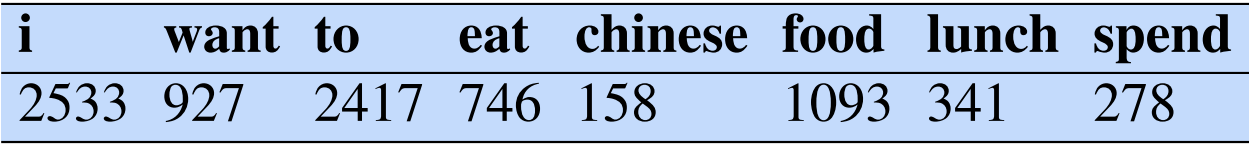
二元单词分布情况表：

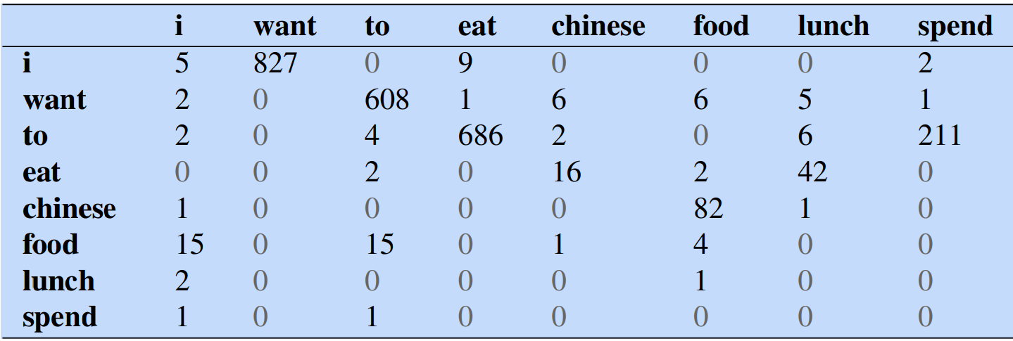
第一行，第二列表示给定前一个词是$“i”$时，当前词为$“want"$的情况一共出现了827次。

频率分布表：

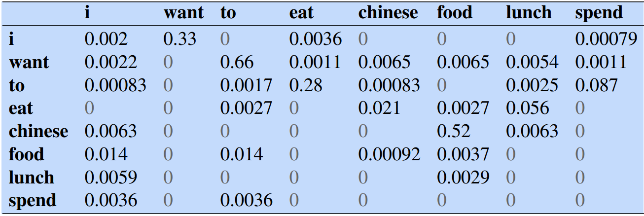
因为我们从表1中知道$"i"$一共出现了2533次，而其后出现“want”的情况一共有827次，所以

$$ \begin{aligned} P(want|i)&=\frac{827}{2533} \\ &\approx0.33 \end{aligned} $$

例如：I want chinese food.

$$ \begin{aligned} p(I\,want\,chinese\,food)&=p(want|I) \cdot p(chinese|want) \cdot p(food|chinese) \\&=0.33 _ 0.0065 _ 0.52 \\&=0.0011154 \end{aligned} $$

第四节 代码示例

pip install nltk

import nltk
from nltk.util import ngrams
from nltk.tokenize import word_tokenize

# 文本
text = "Natural Language Processing with Python is amazing"

# 将字符串按单词拆分
words = word_tokenize(text)

# 创建 bigrams (2-grams)
bigrams = list(ngrams(words, 2))
print("Bigrams:", bigrams)

# 创建 trigrams (3-grams)
trigrams = list(ngrams(words, 3))
print("Trigrams:", trigrams)

# 创建 n-grams (you can specify any n)
n = 4
n_grams = list(ngrams(words, n))
print(f"{n}-grams:", n_grams)

第五节 n-gram的优缺点

n-gram 的优点：

1. 简单直观：模型结构相对简单，易于理解和实现。
2. 对语言的局部特征有较好的捕捉能力。

n-gram 的缺点：

1. 数据稀疏问题：对于长序列或罕见的组合，可能出现数据稀疏导致模型不准确。
2. 缺乏对上下文的整体理解：无法充分考虑句子的整体语义关系。
3. 维度较高：随着 n 的增大，模型的维度会迅速增加，导致计算和存储成本增加。

第六节 n-gram的一些应用例子

第七节 可靠性与可区别性

假设没有计算和存储限制，$n$ 是不是越大越好呢？

早期由于计算性能的限制，一般最大取到$n=4$，如今，即使$n>10$也没有问题。但随着$n$的增大，模型的性能增大却不显著，这其中涉及到可靠性与可区别性的问题。

参数越多，模型的可区别性越好，但同时可靠性却在下降——这是因为语料的规模是有限的，导致$count(W)$的实例数量不够，从而降低了可靠性。此外，还需要考虑不同领域或任务中对$n$的选择差异，以及如何根据具体情况进行权衡。

为了解决可靠性下降的问题，可以采用合适的平滑技术、数据增强方法等。在实际应用中，需要综合考虑性能、计算资源、实际效果等多方面因素来确定合适的$n$值。同时，还应关注$n$与模型复杂度、泛化能力之间的关系。随着研究的深入，关于$n$的选择以及其与模型性能的关系也在不断发展，有很多相关的研究进展和最新观点值得我们进一步探讨。

第八节 停用词

停用词（Stopwords）是在文本处理中经常出现但对特定任务没有实际意义的词。这些词通常是高频词，像连词、冠词、介词、代词等，在句子中起到语法功能，但对文本分析任务（如文本分类、情感分析、信息检索等）没有实际贡献。常见的停用词包括“的”、“是”、“在”、“和”、“了”、“有”等。

为什么要去除停用词：

1. 减少噪音： 停用词在文本中出现频率高，但对区分文本内容的有用性低，去除它们可以减少噪音，提高模型的准确性。
2. 提高效率： 去除停用词可以减少文本的维度，从而加快计算速度。
3. 聚焦重要信息： 保留有意义的词汇，有助于模型更好地理解和处理文本中的重要信息。

如何去除停用词：

在自然语言处理（NLP）任务中，通常会使用停用词列表（stopwords list）来识别并去除这些词。以下是如何在Python中使用NLTK库去除停用词的示例代码：

安装NLTK库：

如果还没有安装NLTK库，可以使用以下命令进行安装：

pip install nltk

代码示例：

import nltk
from nltk.corpus import stopwords
from nltk.tokenize import word_tokenize

# 下载停用词列表
nltk.download('stopwords')
nltk.download('punkt')

# 示例文本
text = "Natural Language Processing with Python is amazing and it provides great tools."

# 分词
words = word_tokenize(text)

# 获取英语的停用词列表
stop_words = set(stopwords.words('english'))

# 去除停用词
filtered_words = [word for word in words if word.lower() not in stop_words]

print("Original words:", words)
print("Filtered words:", filtered_words)

代码解释：

1. 下载停用词列表和分词器数据： nltk.download('stopwords') 和 nltk.download('punkt') 下载停用词列表和分词器所需的数据。
2. 分词： 使用 word_tokenize 将文本分割成单词。
3. 获取停用词列表： 使用 stopwords.words('english') 获取英语的停用词列表，并将其转换为集合（set）以提高查找效率。
4. 去除停用词： 使用列表推导式遍历分词后的单词，保留不在停用词列表中的单词。

示例输出：

Original words: ['Natural', 'Language', 'Processing', 'with', 'Python', 'is', 'amazing', 'and', 'it', 'provides', 'great', 'tools', '.']
Filtered words: ['Natural', 'Language', 'Processing', 'Python', 'amazing', 'provides', 'great', 'tools', '.']

常见停用词库：

除了NLTK，还有其他一些常见的停用词库：

1. spaCy: 另一个广泛使用的NLP库，包含多种语言的停用词列表。
2. gensim: 专注于主题建模和文档相似度分析，也提供停用词列表。

自定义停用词：

在实际应用中，标准停用词列表可能不足以满足特定任务的需求，您可能需要根据具体的应用场景自定义停用词列表。例如，添加特定领域的术语，或者删除某些对任务有意义的词。

custom_stop_words = set(stopwords.words('english')).union({'example', 'anotherword'})
filtered_words_custom = [word for word in words if word.lower() not in custom_stop_words]

通过去除停用词，可以使文本处理任务更加高效和准确。

第九节 OOV 问题

$OOV$即“超出词汇表”（Out Of Vocabulary），指的是在序列中出现了词表外的词，这些词也被称为未登录词。在测试集或验证集中，可能会出现一些在训练集中从未出现过的词。

一般的解决方案如下：

• 设置词频阈值：设定一个特定的词频阈值，只有词频高于该阈值的词才会被纳入词表。

• 替换为特殊符号：将所有低于阈值的词替换为$UNK$（一个特殊符号）。

对于统计语言模型和神经语言模型来说，它们在处理 OOV 问题时的方式较为相似。但值得注意的是，OOV 问题仍然是语言模型面临的一个重要挑战，需要不断探索和创新更有效的解决方法来提高模型的性能和泛化能力。此外，还可以考虑结合上下文信息来更好地处理 OOV 问题，以及利用外部知识库或词典来辅助解决。

第十节 平滑处理

n-gram 平滑处理是一种在 n-gram 模型中用于处理未出现的 n 元语法的技术。其基本思想是为所有可能出现的字符串分配一个非零的概率值，以避免在评估测试语料中的句子时出现概率为 0 的情况。

方法名称	解释
加 1 法（additive smoothing）	假设每个 n 元语法出现的次数比实际出现次数多一次。
减值法/折扣法（discounting）	通过对观察到的频率进行折扣来调整概率估计。
拉普拉斯平滑（Laplace Smoothing）	在分子和分母上分别加 1，强制让所有 n-gram 至少出现一次。
Add-one 拉普拉斯平滑	在拉普拉斯平滑基础上，加上一个小于 1 的常数 K。
Add-K 拉普拉斯平滑	与 Add-one 拉普拉斯平滑类似，但加上的常数 K 可以是任意值。
古德-图灵（Good-Turing）估计法	用观察计数较高的 n 元语法数重新估计概率量的大小，并指派给零计数或较低计数的 n 元语法。

这些方法都有其优缺点，具体使用哪种方法取决于具体的应用场景和数据特点。在实际应用中，通常需要根据实验结果进行调整和优化，以获得更好的性能。

第十一节 本章小结

该语言模型只看当前词的前 $n-1$ 个词对当前词的影响。

因此该模型的优势为：

• 该模型包含了前 $n-1$ 个词所能提供的全部信息，这些词对当前词的出现具有很强的约束能力；
• 只看前 $n-1$ 个词而非所有词，所以使得模型的效率较高；

该模型也有很多缺陷：

• $n-gram$ 语言模型无法建模更远的关系，语料的不足使得无法训练更高阶的语言模型（通常 $n=2$ 或 $3$ ）
• 该模型无法建模出词与词之间的相似度，比如”白色汽车”和”白色轿车”
• 训练语料中有些 n 元组没有出现过，其对应的条件概率为0，导致计算一整句话的概率为0

第二章 神经网络语言模型(NPLM)

第一节 NPLM介绍

“A Neural Probabilistic Language Model”（Bengio等人，2003）是一个经典的神经概率语言模型，它在某种程度上沿用了N-gram模型的思路，但通过神经网络来建模语言的概率分布，从而克服了传统N-gram模型的一些限制。

虽然N-gram模型和神经概率语言模型都是用于建模语言的概率分布，但它们的建模方式有所不同：

1. N-gram模型：

   • N-gram模型是一种基于统计的语言模型，它假设当前词的出现只与前面的N-1个词相关。

• N-gram模型通过统计语料库中词的频率和它们之间的组合来计算概率，通常使用基于频率的方法来估计概率。

2. 神经概率语言模型：

   • 神经概率语言模型则利用神经网络来建模语言的概率分布，通过学习词之间的语义关系和上下文信息来预测下一个词的概率。
   • 这种模型可以捕捉更复杂的语言模式和关系，因为神经网络具有更强大的表达能力，而且可以处理更长的上下文信息。

   虽然神经概率语言模型在一定程度上借鉴了N-gram模型的思路，但它通过神经网络来学习更复杂的语言模式和关系，从而能够在语言建模任务中取得更好的性能。”Bengio et al., 2003”的工作为神经概率语言模型的发展奠定了重要的基础，并为后续的研究提供了启示。

第二节 条件概率公式

泛化形式：

$$ p(w|context(w))=g(i*w,V*{context}) $$

其中 $g$ 表示神经网络，$i_w$ 为 $w$ 在词表中的序号，$context(w)$ 为 $w$ 的上下文，$V_{context}$ 为上下文构成的特征向量。$V_{context}$ 由上下文的词向量进一步组合而成，通常使用拼接的方式，即将上下文中每个词的词向量连接起来，以形成一个更丰富的上下文表示。

$w$ 的上下文 $context(w)$ 是 $w$ 的前 $n-1$ 个词得到的，而 $V_{context}$ 是由 $n-1$ 个词的词向量拼接而成，即

$$ p(w*k|w^{k-1}*{k-n+1})=g(i*{w_k},[c(w*{k-n+1});...;c(w\_{k-1})]) $$

​

其中 $n$ 代表窗口大小，$k$ 代表是当前位置， $c(w)$ 表示 $w$ 的词向量。将上下文的词向量拼接起来可以捕捉更丰富的上下文信息，帮助模型更好地预测下一个单词。

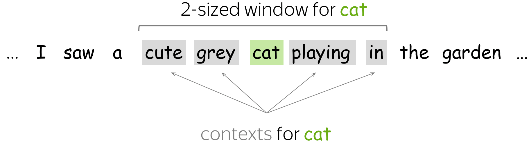
例如：

如上图所示，为了得到 $n-1=2$ 个单词，则需要将$n=3$。

• 所以 $k = 6$ 且 $n =3$：

  • 当前单词是 $w_6$。
  • 上下文单词是 $w_4, w_5$（总共两个，即 $n-1$ 个单词）。

• 所以， $w^{k-1}_{k-n+1}$ 即 $w_4, w_3$。

• 公式会看作 $p(w_5 \mid w_3, w_4) = g(i_{w_5}, [c(w_3); c(w_4)])$。

不同的神经语言模型中 $context(w)$ 的表示方式可能不同，例如 $Word2Vec$ 中的 $CBoW$ 模型将上下文中的词向量简单平均作为上下文表示，而其他模型可能使用不同的方法。这些不同的表示方法会影响模型对上下文信息的理解和利用。

每个训练样本是形如 $(context(w), w)$ 的二元对，其中 $context(w)$ 取 $w$ 的前 $n-1$ 个词；当不足 $n-1$ 个词时，可以使用特殊符号填充。

同一个网络只能训练特定的 $n$，不同的 $n$ 需要训练不同的神经网络。

第三节 网络结构与计算过程

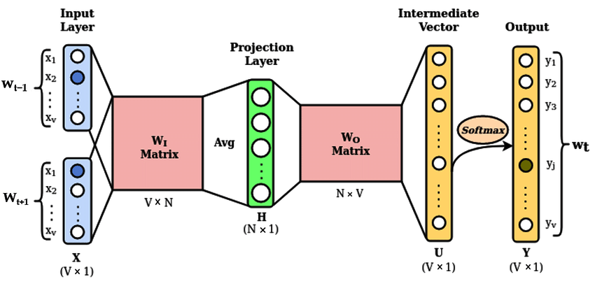
NPLM神经语言模型的网络结构：

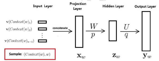
在NPLM（Neural Probabilistic Language Model）中，在进入投影层之前进行concatenate操作的目的是将输入的词向量连接在一起，以提供更丰富的上下文信息。

具体来说，这个concatenate操作通常是将多个词的词向量按照顺序连接在一起，形成一个更长的向量。这个连接的过程可以将当前词的词向量与其前面的若干个词的词向量结合起来，从而提供更多的上下文信息给模型。

训练样本：$(Context(w), w)$ 包括前$n-1$个词分别的向量，假定每个词向量大小 $m$

投影层：$(n-1) * m$ 首尾拼接起来的大向量

输出：$y_w=(y_{w_1}, y_{w_2},...,y_{w_n})^T$

表示上下文为 $Context(w)$ 时，下一个词恰好为词典中第$i$个词的概率。

归一化：$p(w|Context(w))=\frac{e^{y_{w,i_w}}}{\sum_{i=1}^Ne^{y_{w,i}}}$

【输入层】首先，将 $context(w)$ 中的每个词映射为一个长为 $m$ 的词向量，词向量再训练开始时是随机的，并参与训练；

【投影层】将所有上下文词向量拼接为一个长向量，作为 $w$ 的特征向量，该向量的维度为 $m(n-1)$

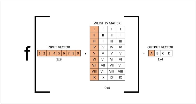
投影层的运算是通过矩阵乘法来实现的，其目的是将输入的词向量映射到隐藏层的表示空间。

假设投影层的输入为一个向量 $x$ ，维度为 $d_{input}$ ，其中 $d_{input}$ 是词向量的维度；投影层的权重矩阵为$W$，维度为$d_{input} * d_{hidden} $，其中 $d_{hidden}$ 是隐藏层的维度。则投影层的输出 $h$ 计算方式如下：

$$h=x \cdot W$$

其中 $\cdot$ 表示矩阵乘法操作。

在这个过程中，输入向量 $x$ 中的每个元素分别与权重矩阵 $W$ 中对应位置的元素相乘，然后将所有结果相加，得到隐藏层的输出向量 $h$，这个过程实现了将输入词向量映射到隐藏层表示空间的功能，同时通过学习权重矩阵 $W$，模型可以从数据中学习到更有效的特征表示。

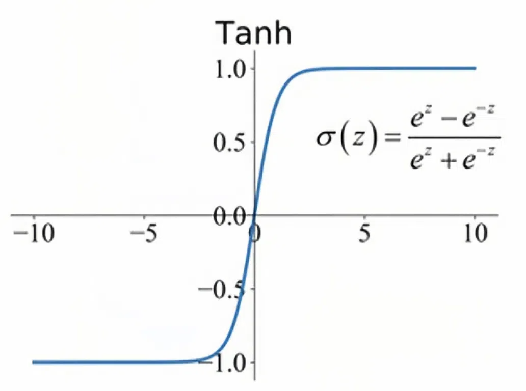
【隐藏层】拼接后的向量会经过一个规模为 $h$ 的隐藏层，该隐层使用的激活函数为 $tanh$

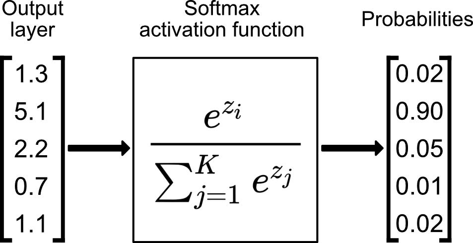
【输出层】最后会经过一个规模为 $N$ 的 $Softmax$ 输出层，从而得到词表中每一个词作为下一个词的概率分布。

其中 $m，n，h$ 为超参数，$N$ 为词表大小，视训练集规模而定，也可以人为设置阈值

训练时，使用交叉熵作为损失函数

当训练完成时，就得到了 NPLM 神经语言模型，以及副产品词向量

整个模型可以概括为如下公式：

$$ y=U \cdot tanh(Wx + p) + q $$

第四节 模型参数的规模与运算量

模型的超参数：$m，n，h，N$

• $m$ 为词向量的维度，通常在 $10^1 \sim 10^2$ 之间。
• $n$ 为 $n$-gram 的规模，一般小于 $5$。
• $h$ 为隐藏层的单元数，一般在 $10^2$。
• $N$ 为词表的数量，一般在 $10^4 \sim 10^5$，甚至 $10^6$。

网络参数包括两部分：

• 词向量 $C$：一个 $N*m$ 的矩阵，其中 $N$ 为词表大小，$m$ 为词向量的维度。

• 神经网络的参数：

  • $W$：一个 $h * m(n-1)$ 的矩阵，用于连接输入层和隐藏层。
  • $p$：一个 $h * 1$ 的矩阵，用于隐藏层的偏置。
  • $U$：一个 $N * h$ 的矩阵，用于连接隐藏层和输出层。
  • $q$：一个 $N * 1$ 的矩阵，用于输出层的偏置。

模型的运算量主要集中在隐藏层和输出层的矩阵运算，以及 Softmax 的归一化计算。具体来说，隐藏层的计算涉及矩阵乘法和偏置的加法，而输出层的计算涉及矩阵乘法和 Softmax 函数的应用。这些计算的复杂度随着隐藏层单元数和词表大小的增加而增加。

未来的相关研究主要集中在优化模型的计算效率和性能方面，其中包括对模型参数和计算过程的优化，以及对算法和数据结构的改进。例如，$Word2Vec$ 的工作就是在这个方向上取得了重要进展。

第五节 NPLM与N-gram模型对比

相比传统的 N-gram 模型（N-gram Language Model），神经概率语言模型（Neural Probabilistic Language Model，NPLM）具有几个显著的优势：

1. 考虑了长程依赖性： N-gram 模型只考虑了有限的上下文窗口，无法很好地捕捉长程的依赖关系。而 NPLM 利用神经网络结构，可以更好地建模长程依赖关系，因为神经网络能够学习到更复杂的语言结构和模式，从而更好地理解文本中的语义信息。

2. 词嵌入的学习： NPLM 使用词嵌入（Word Embeddings）来表示单词，而不是简单地将单词映射到离散的整数索引。这使得模型能够通过训练数据自动学习单词之间的语义相似性，从而更好地处理同义词、近义词等语言现象。

3. 参数共享： 在 N-gram 模型中，参数量随着 $n$ 的增加呈指数级增长，容易造成维度灾难（Curse of Dimensionality）。而 NPLM 中采用参数共享的方式，通过共享权重矩阵等方法，有效地降低了模型参数的数量，提高了模型的训练效率。

4. 泛化能力： NPLM 在大规模数据集上的表现通常比 N-gram 模型更好，尤其是在处理未见过的词或者稀有词时，因为它能够通过词嵌入学习到更加通用的语言模式，从而具有更好的泛化能力。

5. 端到端的训练： NPLM 可以通过端到端的方式进行训练，即将文本数据作为输入，直接学习文本的概率分布，而不需要手工设计特征或者预处理文本。这使得模型更加灵活和通用，可以适应不同领域和任务的需求。

第六节 代码实现

import torch.nn as nn

# 定义神经概率语言模型（NPLM）
class NPLM(nn.Module):
    def __init__(self):
        super(NPLM, self).__init__()

        # 定义一个词嵌入层
        self.C = nn.Embedding(voc_size, embedding_size)

        # 第一个线性层，其输入大小为 n_step * embedding_size，输出大小为 n_hidden
        self.linear1 = nn.Linear(n_step * embedding_size, n_hidden)

        # 第二个线性层，其输入大小为 n_hidden，输出大小为 voc_size，即词汇表大小
        self.linear2 = nn.Linear(n_hidden, voc_size)

  # 定义前向传播过程
    def forward(self, X):
        # 输入数据 X 张量的形状为 [batch_size, n_step]
        X = self.C(X)  # 将 X 通过词嵌入层，形状变为 [batch_size, n_step, embedding_size]

    # 形状变为 [batch_size, n_step * embedding_size]
        X = X.view(-1, n_step * embedding_size)

        # 通过第一个线性层
        X = self.linear1(X)

        # 应用 ReLU 激活函数
        hidden = torch.tanh(X)           # hidden 张量形状为 [batch_size, n_hidden]

        # 通过第二个线性层得到输出
        output = self.linear2(hidden)    # output 形状为 [batch_size, voc_size]

        return output                    # 返回输出结果

第三章 词向量

词向量（Word vectors），也称为词嵌入（Word embeddings），是将单词映射到一个连续的实数向量空间中的表示形式。在自然语言处理（NLP）中，词向量是一种用来表示单词的方法，其目的是捕捉单词之间的语义相似性和语法关系，以便计算机能够更好地理解和处理文本数据。

第一节 独热编码

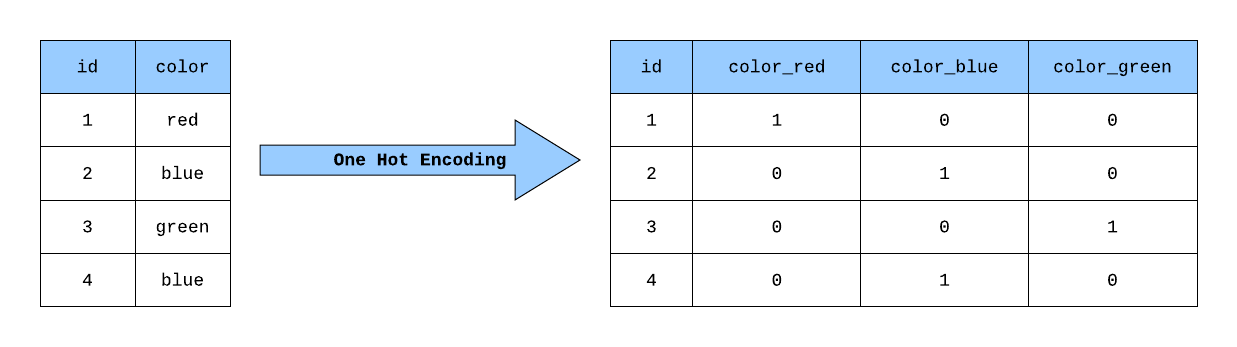
“One-hot representation”（独热表示）是一种常见的向量表示方法，通常用于将分类变量转换为数值表示。在这种表示方法中，每个分类变量被表示为一个只有一个元素为1，其余元素为0的向量。

具体来说，如果有 $n$ 个不同的分类值，那么每个分类值就被映射为一个长度为 $n$ 的向量，其中只有对应分类值的位置上的元素为1，其余位置上的元素都为0。这样，每个分类值都被表示为了一个唯一的向量。

举例来说，假设有一个包含三个分类值的变量，分别为”A”、”B”和”C”。使用独热表示，这三个分类值可以被映射为以下向量：

• “A”：[1, 0, 0]
• “B”：[0, 1, 0]
• “C”：[0, 0, 1]

这种表示方法的优点是简单明了，每个分类值都被唯一地表示为一个向量，不存在歧义。但是，对于具有大量不同取值的分类变量来说，独热表示会导致向量维度过高，可能会造成存储和计算上的浪费。

第二节 Word2Vec

Word2vec 是自然语言处理（NLP）中的一项技术，用于获取单词的向量表示。这些向量通过捕捉周围单词的信息，反映单词的语义。Word2vec 通过对大型语料库中的文本进行建模，估计这些表示。经过训练，这样的模型可以检测同义词或为部分句子建议附加单词。Word2vec 由 Tomáš Mikolov 和 Google 的同事开发，于 2013 年发布。

独热编码虽然可以将文本转化为数字形式，但存在数据稀疏和维度灾难等问题。Word2vec 是对独热编码的一种改进和发展。它用低维、稠密的向量来表示单词，相较于独热编码能更好地捕捉单词的语义信息，向量之间的距离也能反映单词语义的相似度。它解决了独热编码的一些弊端，在自然语言处理任务中表现出更好的性能和效率，是对传统独热编码处理文本方式的一种优化和创新。

Word2vec 主要有两种模型，连续词袋模型（CBOW） 和 跳字模型（Skip-gram）。通过大规模语料的训练，Word2vec 可以将每个单词映射到一个低维空间的向量上。这些向量具有一些良好的特性，比如语义相似的单词在向量空间中距离较近。这样就使得计算机可以通过对这些向量的操作和计算来处理文本，实现诸如文本分类、情感分析、机器翻译等任务。它极大地促进了自然语言处理中对词汇语义的理解和处理能力的提升。

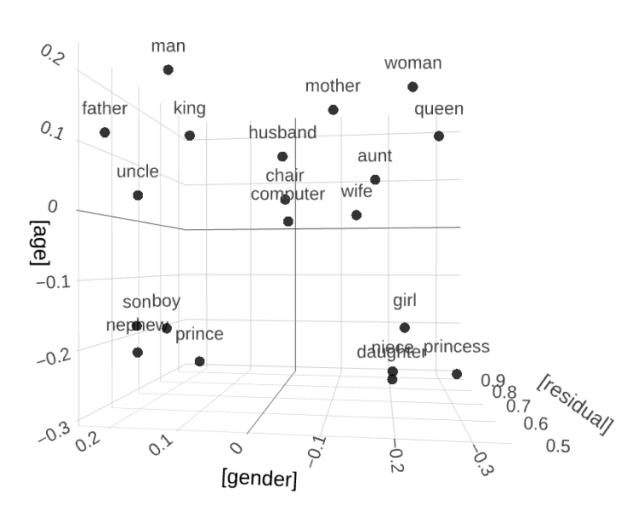
如下图词向量模型是一种将词的语义映射到向量空间的技术，而且词与词之间可以通过计算余弦相似度来看两个词的语义是否相近，显然 King 和 Man 两个单词语义更加接近，而且通过实验我们知道

$$ King-Man+Woman=Queen $$

3.2.1 CBoW(连续词袋模型)

3.2.1.1 CBoW介绍

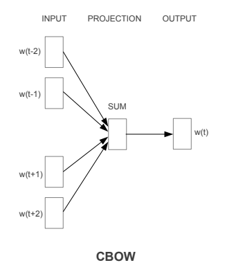
CBoW（Continuous Bag-of-Words，连续词袋模型）是 Word2Vec 中的一种模型。

CBoW 的基本原理是利用一个词的上下文来预测该词。它以某个词周围的若干个词作为输入，目标是预测中间的那个词。在训练过程中，模型通过不断调整参数来最小化预测误差，从而学习到词与词之间的语义关系，并将每个词表示为一个固定长度的向量。

例如，给定一个句子“我爱自然语言处理”，对于“自然”这个词，CBoW 会以“我”“爱”“语言”“处理”这些词作为输入来预测“自然”。通过大量语料的训练，得到的词向量能够在一定程度上反映词的语义特征，比如语义相近的词在向量空间中距离较近。这样就为后续的自然语言处理任务提供了有力的支持。

网络结构如下：

3.2.1.2 CBoW计算过程

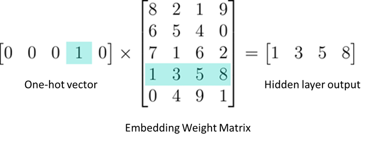
在连续词袋模型（CBoW）中，输入的是每个词的独热编码，输出的是独热编码与权重矩阵相乘的向量。

然后向量与向量相加是将它们对应的元素分别相加。

假设我们有两个向量 A 和 B，A = [a1, a2, a3,…]，B = [b1, b2, b3,…]，那么它们相加后的向量 C = [a1 + b1, a2 + b2, a3 + b3,…]。
例如，如果 A = [1, 2, 3]，B = [4, 5, 6]，那么相加后的向量 C = [1 + 4, 2 + 5, 3 + 6] = [5, 7, 9]。

具体过程：

1. 输入：中心词周围若干个上下文词的独热编码向量。假设上下文窗口大小为 $2c$，则输入为 $2c$ 个上下文词的独热编码向量。

2. 前向传播：

   • 投影层：将这些独热编码向量通过权重矩阵 $W$ 映射到隐藏层。假设词汇表大小为 $V$，隐藏层维度为 $N$，则权重矩阵 $W$ 是一个 $V×N$ 的矩阵。对于每个上下文词的独热编码向量 $x_i$（其中 $i$ 从 1 到 $2c$），映射到隐藏层得到隐藏层向量 $h_i$：$h_i = W^T x_i$
   • 累加求和：将所有上下文词映射到隐藏层的向量进行累加，然后取平均，得到投影层向量 $h$：$h = \frac{1}{2c} \sum_{i=1}^{2c} h_i$

3. 映射到输出层：通过另一个权重矩阵 $W'$ 将投影层向量 $h$ 映射到输出层，得到输出层向量 $u$：$u = W' h$
   然后通过 softmax 函数将 $u$ 转换为输出概率分布向量 $y$：$y = softmax(u)$

4. 损失计算：使用交叉熵损失函数计算预测的输出 $y$ 与实际中心词的独热编码向量之间的差异。损失函数 $L$ 通常为：$L = - \log(y_{target})$ 其中 $y_{target}$ 是实际中心词在输出概率分布中的概率。

5. 反向传播：依据损失值，通过梯度下降等优化算法更新权重矩阵 $W$ 和 $W'$。具体步骤为：

   • 计算输出层的梯度，并更新权重矩阵 $W'$：$W' = W' - \eta \cdot \frac{\partial L}{\partial W'}$
   • 计算投影层的梯度，并更新权重矩阵 $W$：$W = W - \eta \cdot \frac{\partial L}{\partial W}$

6. 不断迭代训练：重复以上步骤，使用大量文本数据进行训练，以逐渐优化模型参数，得到准确的词向量表示。

示例:

假设词汇表为 [“I”, “like”, “to”, “play”, “football”]，大小为 $V = 5$。假设上下文窗口大小为 2（即前后各两个词），隐藏层维度为 $N = 3$。

输入：”I like to play football” 中的上下文词是 “I”, “to”, “play”, “football”，中心词是 “like”。

独热编码向量：

词	独热编码向量
I	[1,0,0,0,0]
to	[0,0,1,0,0]
play	[0,0,0,1,0]
football	[0,0,0,0,1]

假设权重矩阵 W 和 W' 如下：

$$ W = \begin{bmatrix} 0.1 & 0.2 & 0.3 \\ 0.4 & 0.5 & 0.6 \\ 0.7 & 0.8 & 0.9 \\ 1.0 & 1.1 & 1.2 \\ 1.3 & 1.4 & 1.5 \\ \end{bmatrix} $$ $$ W' = \begin{bmatrix} 0.1 & 0.4 & 0.7 & 1.0 & 1.3 \\ 0.2 & 0.5 & 0.8 & 1.1 & 1.4 \\ 0.3 & 0.6 & 0.9 & 1.2 & 1.5 \\ \end{bmatrix} $$

将输入词映射到隐藏层并求平均：

$$ \begin{aligned} h*I &= W^T \cdot [1, 0, 0, 0, 0]^T = [0.1, 0.2, 0.3] \\h*{to} &= W^T \cdot [0, 0, 1, 0, 0]^T = [0.7, 0.8, 0.9] \\h*{play} &= W^T \cdot [0, 0, 0, 1, 0]^T = [1.0, 1.1, 1.2] \\h*{football} &= W^T \cdot [0, 0, 0, 0, 1]^T = [1.3, 1.4, 1.5] \end{aligned} $$ $$ \begin{aligned} h &= \frac{1}{4}([0.1, 0.2, 0.3] + [0.7, 0.8, 0.9] + [1.0, 1.1, 1.2] + [1.3, 1.4, 1.5]) \\ &= \frac{1}{4}[3.1, 3.5, 3.9] \\ &= [0.775, 0.875, 0.975] \end{aligned} $$

将投影层向量映射到输出层并通过softmax得到概率分布：

$$ \begin{aligned} u &= W' \cdot [0.775, 0.875, 0.975]^T \\&= \begin{bmatrix} 0.1 & 0.4 & 0.7 & 1.0 & 1.3 \\ 0.2 & 0.5 & 0.8 & 1.1 & 1.4 \\ 0.3 & 0.6 & 0.9 & 1.2 & 1.5 \\ \end{bmatrix} \cdot \begin{bmatrix} 0.775 \\ 0.875 \\ 0.975 \\ \end{bmatrix} \\ &= [1.225, 1.6, 1.975, 2.35, 2.725] \end{aligned} $$ $$ \begin{aligned} y &= softmax(u) \\&= \frac{e^{u*i}}{\sum*{j=1}^n e^{u_j}} \end{aligned} $$

首先计算向量$u$中每个元素的指数值：

$$ e^{1.225}\approx3.405 $$ $$ e^{1.6}\approx4.953 $$ $$ e^{1.975}\approx7.202 $$ $$ e^{2.35}\approx10.49 $$ $$ e^{2.725}\approx15.27 $$

然后计算所有指数值的和：

$$ 3.405+4.953+7.202+10.49+15.27=41.32 $$

则$y$的结果为：

$$ y_1=\frac{3.405}{41.32}\approx0.0824 $$ $$ y_2=\frac{4.953}{41.32}\approx0.1201 $$ $$ y_3=\frac{7.202}{41.32}\approx0.1743 $$ $$ y_4=\frac{10.49}{41.32}\approx0.2539 $$ $$ y_5=\frac{15.27}{41.32}\approx0.3701 $$

所以

$$ y\approx[0.0824,0.1201,0.1743,0.2539,0.3701] $$

计算损失并进行反向传播，更新 W 和 W'。

通过这种方式，CBOW 模型可以不断优化词向量，使得相似语义的词在向量空间中距离更近。

CBOW模型的最终输出是一个概率分布向量，我们通常会取该分布中最大概率对应的词作为模型的预测结果。

3.2.1.3 代码实验1

定义语料库：

import torch
from torch import nn
import numpy as np
import matplotlib.pyplot as plt
from sklearn.decomposition import PCA

# 定义语料库
corpus = ['The cat sat on the mat',
          'The dog ran in the park',
          'The bird sang in the tree']

# 将语料库转换为整数序列
tokenizer = {}
for i, text in enumerate(corpus):
    for word in text.split():
        if word not in tokenizer:
            tokenizer[word] = len(tokenizer)
sequences = [[tokenizer[word] for word in text.split()] for text in corpus]
print("将语料库中的单词转换为整数向量后:")
print(sequences)

定义CBOW模型：

# 定义参数
vocab_size = len(tokenizer) + 1
embedding_size = 10
window_size = 2

# 生成上下文目标对
contexts = []
targets = []
for sequence in sequences:
    for i in range(window_size, len(sequence) - window_size):
        context = sequence[i - window_size:i] + sequence[i + 1:i + window_size + 1]
        target = sequence[i]
        contexts.append(context)
        targets.append(target)

# 将上下文和目标转换为 numpy 数组
X = np.array(contexts)

# 定义 PyTorch 模型
class CBOWModel(nn.Module):
    def __init__(self, vocab_size, embedding_size):
        super(CBOWModel, self).__init__()
        self.embedding = nn.Embedding(vocab_size, embedding_size)
        self.linear = nn.Linear(embedding_size, vocab_size)

    def forward(self, x):
        x = self.embedding(x)
        x = x.mean(dim=1)
        x = self.linear(x)
        return x

可视化嵌入：

model = CBOWModel(vocab_size, embedding_size)

# 获取单个词的词嵌入
embeddings = model.embedding.weight.detach().numpy()

# 执行 PCA 以降低嵌入的维度
pca = PCA(n_components=2)
reduced_embeddings = pca.fit_transform(embeddings)

# 可视化嵌入
plt.figure(figsize=(5, 5))
for i, word in enumerate(tokenizer.keys()):
    x, y = reduced_embeddings[i]
    plt.scatter(x, y)
    plt.annotate(word, xy=(x, y), xytext=(5, 2),
                 textcoords='offset points',
                 ha='right', va='bottom')
plt.show()

3.2.1.4 代码实验2

import torch
import torch.nn as nn
import torch.nn.functional as F
import torch.optim as optim
import numpy as np
import urllib.request
from nltk.tokenize import RegexpTokenizer
from nltk.corpus import stopwords
from nltk import word_tokenize
import sklearn
from sklearn.cluster import KMeans
from sklearn.metrics.pairwise import euclidean_distances

# 设置随机种子，确保结果可重复
torch.manual_seed(1)

# 上下文大小
CONTEXT_SIZE = 3
# 嵌入维度
EMBEDDING_DIM = 10

# 测试句子
test_sentence = """Empathy for the poor may not come easily to people who never experienced it. They may blame the victims and insist their predicament can be overcome through determination and hard work.
But they may not realize that extreme poverty can be psychologically and physically incapacitating — a perpetual cycle of bad diets, health care and education exacerbated by the shaming and self-fulfilling prophecies that define it in the public imagination.
Gordon Parks — perhaps more than any artist — saw poverty as “the most savage of all human afflictions” and realized the power of empathy to help us understand it. It was neither an abstract problem nor political symbol, but something he endured growing up destitute in rural Kansas and having spent years documenting poverty throughout the world, including the United States.
That sensitivity informed “Freedom’s Fearful Foe: Poverty,” his celebrated photo essay published in Life magazine in June 1961. He took readers into the lives of a Brazilian boy, Flavio da Silva, and his family, who lived in the ramshackle Catacumba favela in the hills outside Rio de Janeiro. These stark photographs are the subject of a new book, “Gordon Parks: The Flavio Story” (Steidl/The Gordon Parks Foundation), which accompanies a traveling exhibition co-organized by the Ryerson Image Centre in Toronto, where it opens this week, and the J. Paul Getty Museum. Edited with texts by the exhibition’s co-curators, Paul Roth and Amanda Maddox, the book also includes a recent interview with Mr. da Silva and essays by Beatriz Jaguaribe, Maria Alice Rezende de Carvalho and Sérgio Burgi.
""".split()
# 我们应该对输入进行标记，但现在我们忽略这一点
# 构建一个元组列表。每个元组是([ word_i-2, word_i-1 ], 目标单词)

# 根据单词ID获取单词
def get_key(word_id):
    for key, val in word_to_ix.items():
        if(val == word_id):
            print(key)

# 聚类嵌入向量
def cluster_embeddings(filename, nclusters):
    X = np.load(filename)
    kmeans = KMeans(n_clusters=nclusters, random_state=0).fit(X)
    center = kmeans.cluster_centers_
    distances = euclidean_distances(X, center)

    for i in np.arange(0, distances.shape[1]):
        word_id = np.argmin(distances[:, i])
        print(word_id)
        get_key(word_id)

# 读取数据并进行预处理
def read_data(file_path):
    tokenizer = RegexpTokenizer(r'\w+')
    data = urllib.request.urlopen(file_path)
    data = data.read().decode('utf8')
    tokenized_data = word_tokenize(data)
    stop_words = set(stopwords.words('english'))
    stop_words.update(['.', ',', ':', ';', '(', ')', '#', '--', '...', '"'])
    cleaned_words = [i for i in tokenized_data if i not in stop_words]
    return(cleaned_words)

#test_sentence = read_data('https://www.gutenberg.org/files/57884/57884-0.txt')

ngrams = []
for i in range(len(test_sentence) - CONTEXT_SIZE):
    tup = [test_sentence[j] for j in np.arange(i, i + CONTEXT_SIZE)]
    ngrams.append((tup, test_sentence[i + CONTEXT_SIZE]))
# 打印前3个元组，仅供参考
#print(ngrams)

# 构建词汇表
vocab = set(test_sentence)
print("词汇表长度", len(vocab))
word_to_ix = {word: i for i, word in enumerate(vocab)}

# 定义CBOW模型
class CBOWModeler(nn.Module):
    def __init__(self, vocab_size, embedding_dim, context_size):
        super(CBOWModeler, self).__init__()
        self.embeddings = nn.Embedding(vocab_size, embedding_dim)
        self.linear1 = nn.Linear(context_size * embedding_dim, 128)
        self.linear2 = nn.Linear(128, vocab_size)

    def forward(self, inputs):
        embeds = self.embeddings(inputs).view((1, -1))  # -1表示根据数据大小推断该索引的大小
        #print(np.mean(np.mean(self.linear2.weight.data.numpy())))
        out1 = F.relu(self.linear1(embeds))  # 第一层的输出
        out2 = self.linear2(out1)            # 第二层的输出
        #print(embeds)
        log_probs = F.log_softmax(out2, dim=1)
        return log_probs

    # 预测下一个单词
    def predict(self, input):
        context_idxs = torch.tensor([word_to_ix[w] for w in input], dtype=torch.long)
        res = self.forward(context_idxs)
        res_arg = torch.argmax(res)
        res_val, res_ind = res.sort(descending=True)
        res_val = res_val[0][:3]
        res_ind = res_ind[0][:3]
        #print(res_val)
        #print(res_ind)
        for arg in zip(res_val, res_ind):
            #print(arg)
            print([(key, val, arg[0]) for key, val in word_to_ix.items() if val == arg[1]])

    # 冻结某一层的参数
    def freeze_layer(self, layer):
        for name, child in model.named_children():
            print(name, child)
            if(name == layer):
                for names, params in child.named_parameters():
                    print(names, params)
                    print(params.size())
                    params.requires_grad = False

    # 打印模型层的参数
    def print_layer_parameters(self):
        for name, child in model.named_children():
            print(name, child)
            for names, params in child.named_parameters():
                print(names, params)
                print(params.size())

    # 将嵌入写入文件
    def write_embedding_to_file(self, filename):
        for i in self.embeddings.parameters():
            weights = i.data.numpy()
        np.save(filename, weights)

# 损失列表
losses = []
# 定义负对数似然损失函数
loss_function = nn.NLLLoss()
# 初始化模型
model = CBOWModeler(len(vocab), EMBEDDING_DIM, CONTEXT_SIZE)
# 使用随机梯度下降优化器
optimizer = optim.SGD(model.parameters(), lr=0.001)

# 冻结嵌入层
#model.freeze_layer('embeddings')

for epoch in range(400):
    total_loss = 0
    #------- 嵌入层也在这里训练 ----#
    #lookup_tensor = torch.tensor([word_to_ix["poor"]], dtype=torch.long)
    #hello_embed = model.embeddings(lookup_tensor)
    #print(hello_embed)
    # -----------------------------------------------------#

    for context, target in ngrams:
        # 步骤1. 准备传递给模型的输入（即将单词转化为整数索引并将它们包装在张量中）
        context_idxs = torch.tensor([word_to_ix[w] for w in context], dtype=torch.long)
        #print("Context id", context_idxs)

        # 步骤2. 记住torch会累积梯度。在传入新实例之前，需要清除旧实例的梯度
        model.zero_grad()

        # 步骤3. 运行前向传递，获取下一个单词的对数概率
        log_probs = model(context_idxs)
        #print(log_probs)

        # 步骤4. 计算损失函数。（同样，Torch需要将目标单词包装在张量中）
        loss = loss_function(log_probs, torch.tensor([word_to_ix[target]], dtype=torch.long))
        #print(loss)

        # 步骤5. 进行反向传递并更新梯度
        loss.backward()
        optimizer.step()

        # 调用tensor.item()获取1元素张量的Python数值
        total_loss += loss.item()
    print(total_loss)
    losses.append(total_loss)
#print(losses)  # 每次迭代训练数据时，损失都会减少！

# 打印模型层参数
#model.print_layer_parameters()

# 给定n个上下文单词，预测下一个单词
model.predict(['of', 'all', 'human'])
# 将嵌入写入文件
model.write_embedding_to_file('embeddings.npy')
# 对嵌入进行聚类
cluster_embeddings('embeddings.npy', 2)

3.2.2 Skip-gram(跳字模型)

3.2.2.1 Skip-gram介绍

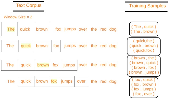
Skip-gram 与 CBoW 相反，它以某个词作为输入，试图预测该词的上下文词。比如对于句子“今天天气真好”，若以“天气”为输入，Skip-gram 模型会尝试预测“今天”“真好”等上下文词。

在 Skip-gram 模型中，通过最大化目标词与其周围词的共现概率来训练模型，从而得到词向量。这种模型更注重捕捉中心词与远距离上下文词之间的关系，对于发现一些不太常见但语义相关的词之间的联系可能更有优势。

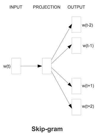
在Skip-Gram架构中，输入是中心词，预测是上下文词。

考虑一个单词数组 W，如果 $W_i$ 是输入（中心单词），则 $W_{i-2}$、$W_{i-1}$、$W_{i+1}$ 和 $W_{i+2}$ 是滑动窗口大小为 $2$ 的上下文单词。

因为神经网络不能直接处理文本，因此所有的词都使用独热编码表示。

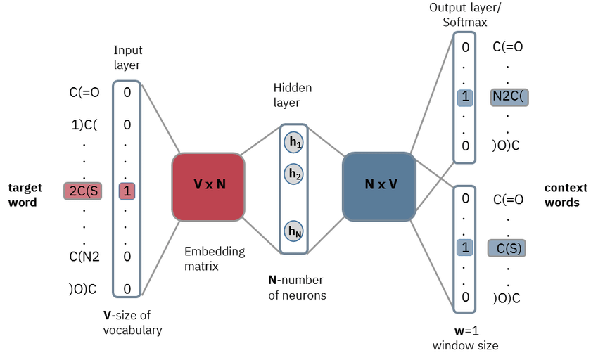
变量	说明
V	文本语料库中唯一单词的数量（词汇）
x	输入层（输入单词的独热编码）
N	神经网络隐藏层中的神经元数量
W	输入层和隐藏层之间的权重
W’	隐藏层和输出层之间的权重
y	Softmax 输出层，具有词汇表中每个单词的概率

3.2.2.2 Skip-gram计算过程

1. 输入：一个中心词的独热编码向量 $x$。

2. 前向传播：

   • 隐藏层：通过权重矩阵 $W$ 将输入层（中心词的独热编码向量 $x$）映射到隐藏层，得到隐藏层向量 $h$。计算公式为 $h = W^T \cdot x$。
   • 输出层：再通过权重矩阵 $W'$ 将隐藏层向量 $h$ 映射到输出层，得到输出层向量 $u$，计算公式为 $u = W' \cdot h$。然后通过softmax函数将 $u$ 转换为输出概率分布向量 $y$，即 $y = softmax(u)$。

3. 损失计算：通常使用交叉熵损失函数来计算预测的输出 $y$ 与实际期望输出（即中心词的上下文词的独热编码向量）的差异。对于每个上下文词，损失为 $L = - log(y_i)$，其中 $y_i$ 是上下文词在输出概率分布中的概率。

4. 反向传播：根据损失计算结果，通过反向传播算法计算梯度，并使用梯度下降法等优化算法来更新权重矩阵 $W$ 和 $W'$。更新公式如下：

   • 更新 $W'$：$W' = W' - η * ∇W' L$
   • 更新 $W$：$W = W - η * ∇W L$

5. 重复：不断重复以上过程，对大量文本数据进行训练，以优化模型参数，得到准确的词向量表示。

具体例子:

Skip-gram模型的计算过程：假设我们有一个小的词汇表，包括 5 个词：[ “I”, “like”, “to”, “play”, “football” ]，词汇表的大小为 $V = 5$。我们选择的隐藏层的维度为 $N = 3$。假设我们正在训练模型，其中中心词是 “like”，上下文词是 [“I”, “to”]。

输入:

中心词 “like” 的独热编码向量 $x$：

$$ x = \begin{bmatrix} 0 \\ 1 \\ 0 \\ 0 \\ 0 \\ \end{bmatrix} $$

前向传播:

隐藏层:

权重矩阵 $W$ 的大小是 $V×N$，假设 $W$ 的值如下：

$$ W = \begin{bmatrix} 0.1 & 0.2 & 0.3 \\ 0.4 & 0.5 & 0.6 \\ 0.7 & 0.8 & 0.9 \\ 1.0 & 1.1 & 1.2 \\ 1.3 & 1.4 & 1.5 \\ \end{bmatrix} $$

计算隐藏层向量 $h$：

$$ \begin{aligned} h &= W^T \cdot x \\&= \begin{bmatrix} 0.1 & 0.4 & 0.7 & 1.0 & 1.3 \\ 0.2 & 0.5 & 0.8 & 1.1 & 1.4 \\ 0.3 & 0.6 & 0.9 & 1.2 & 1.5 \\ \end{bmatrix} \cdot \begin{bmatrix} 0 \\ 1 \\ 0 \\ 0 \\ 0 \\ \end{bmatrix} \\&= \begin{bmatrix} 0.4 \\ 0.5 \\ 0.6 \\ \end{bmatrix} \end{aligned} $$

输出层:
权重矩阵 $W'$ 的大小是 $N×V$，假设 $W'$ 的值如下：

$$ W' = \begin{bmatrix} 0.1 & 0.2 & 0.3 & 0.4 & 0.5 \\ 0.6 & 0.7 & 0.8 & 0.9 & 1.0 \\ 1.1 & 1.2 & 1.3 & 1.4 & 1.5 \\ \end{bmatrix} $$

计算输出层向量 $u$：

$$ \begin{aligned} u &= W' \cdot h \\&= \begin{bmatrix} 0.1 & 0.2 & 0.3 & 0.4 & 0.5 \\ 0.6 & 0.7 & 0.8 & 0.9 & 1.0 \\ 1.1 & 1.2 & 1.3 & 1.4 & 1.5 \\ \end{bmatrix} \cdot \begin{bmatrix} 0.4 \\ 0.5 \\ 0.6 \\ \end{bmatrix} \\&= \begin{bmatrix} 0.1*0.4 + 0.2*0.5 + 0.3 * 0.6 \\ 0.6*0.4 + 0.7*0.5 + 0.8 * 0.6 \\ 1.1*0.4 + 1.2*0.5 + 1.3 * 0.6 \\ \end{bmatrix} \\&= \begin{bmatrix} 0.38 \\ 1.07 \\ 1.76 \\ 2.45 \\ 3.14 \\ \end{bmatrix} \end{aligned} $$

通过softmax函数将 $u$ 转换为输出概率分布向量 $y$：

$$ y = softmax(u) $$ $$ y*i = \frac{e^{u_i}}{\sum*{j} e^{u_j}} $$

计算 softmax 输出：

$$ \begin{aligned} y &= \begin{bmatrix} \frac{e^{0.38}}{e^{0.38} + e^{1.07} + e^{1.76} + e^{2.45} + e^{3.14}} \\ \frac{e^{1.07}}{e^{0.38} + e^{1.07} + e^{1.76} + e^{2.45} + e^{3.14}} \\ \frac{e^{1.76}}{e^{0.38} + e^{1.07} + e^{1.76} + e^{2.45} + e^{3.14}} \\ \frac{e^{2.45}}{e^{0.38} + e^{1.07} + e^{1.76} + e^{2.45} + e^{3.14}} \\ \frac{e^{3.14}}{e^{0.38} + e^{1.07} + e^{1.76} + e^{2.45} + e^{3.14}} \end{bmatrix} \\&=\begin{bmatrix} 0.03257365 \\ 0.06499535 \\ 0.12949669 \\ 0.25814505 \\ 0.51478926 \end{bmatrix} \end{aligned} $$

损失计算:

假设上下文词是 “I” 和 “to”。它们的独热编码向量分别是 $[1, 0, 0, 0, 0]$ 和 $[0, 0, 1, 0, 0]$。

计算每个上下文词的交叉熵损失：

对于 “I”：

$$ L*{I} = - \log(y*{I}) $$

对于 “to”：

$$ L*{to} = - \log(y*{to}) $$

总损失：

$$ L = L*{I} + L*{to} $$

反向传播:

通过反向传播算法计算梯度，并使用梯度下降法更新权重矩阵 $W$ 和 $W'$。更新公式如下：

更新 $W'$：

$$ W' = W' - \eta \cdot \frac{\partial L}{\partial W'} $$

更新 $W$：

$$ W = W - \eta \cdot \frac{\partial L}{\partial W} $$

重复:

不断重复以上过程，使用大量文本数据进行训练，以优化模型参数，得到准确的词向量表示。

通过上述步骤，你可以清晰地看到Skip-gram模型如何通过中心词预测上下文词，并通过优化损失函数来调整模型参数。最终的目标是通过训练，得到准确的词向量，使得在语义上相似的词在向量空间中距离更近。

梯度下降更新公式过程示例:

为了更详细地探讨如何通过梯度下降更新权重矩阵 $W'$，以便你能更好地理解反向传播的具体过程。我们将使用之前的例子来说明。

权重矩阵 $W'$ 的更新公式为：

$$ W' = W' - \eta \cdot \frac{\partial L}{\partial W'} $$

其中：

• $\eta$ 是学习率。
• $\frac{\partial L}{\partial W'}$ 是损失函数 $L$ 对权重矩阵 $W'$ 的梯度。

计算梯度

1. 前向传播：

   • 输入中心词的独热编码向量 $x$。
   • 计算隐藏层向量 $h$：$h = W^T \cdot x$
   • 计算输出层向量 $u$：$u = W' \cdot h$
   • 计算输出概率分布 $y$：$y = softmax(u)$

2. 损失计算：

   • 假设上下文词的独热编码向量为 $t$，损失函数为交叉熵损失：$L = - \sum_{i} t_i \log(y_i)$

3. 反向传播：

   • 计算输出层的误差 $\delta$：$\delta = y - t$

• 计算损失函数对 $W'$ 的梯度 $\frac{\partial L}{\partial W'}$：$\frac{\partial L}{\partial W'} = \delta \cdot h^T$

更新权重矩阵 $W'$

假设 $W'$ 的维度为 $N×V$（在我们的例子中，$N=3$ 和 $V=5$）。为了计算 $\frac{\partial L}{\partial W'}$，我们需要以下步骤：

1. 计算输出层误差：

   • 上文计算得到的 $y$ 是 $softmax(u)$ 的输出。
   • 假设上下文词 “I” 和 “to” 的独热编码向量分别为 $[1, 0, 0, 0, 0]$ 和 $[0, 0, 1, 0, 0]$。那么对应的误差分别为：

   对于 “I”：

$$ \delta\_{I} = y - [1, 0, 0, 0, 0] $$

对于 “to”：

$$ \delta\_{to} = y - [0, 0, 1, 0, 0] $$

2. 计算梯度：
   • 计算对于每个上下文词的梯度，然后取平均值。
   • 我们这里假设批处理包含两个上下文词。

$$ \frac{\partial L}{\partial W'}_{I} = \delta_{I} \cdot h^T $$ $$ \frac{\partial L}{\partial W'}_{to} = \delta_{to} \cdot h^T $$

3. 累加求平均：
   • 对于批处理中的所有上下文词，累加它们的梯度并求平均。

$$ \frac{\partial L}{\partial W'} = \frac{1}{2} \left( \frac{\partial L}{\partial W'}_{I} + \frac{\partial L}{\partial W'}_{to} \right) $$

4. 更新权重：
   • 使用学习率 $\eta$ 更新 $W'$。

$$ W' = W' - \eta \cdot \frac{\partial L}{\partial W'} $$

示例计算:

假设我们有以下具体数值：

• $y$（softmax输出）为 $[0.1, 0.3, 0.2, 0.15, 0.25]$。
• 上下文词 “I” 的独热编码向量为 $[1, 0, 0, 0, 0]$。
• 上下文词 “to” 的独热编码向量为 $[0, 0, 1, 0, 0]$。
• 学习率 $\eta = 0.01$。
• 隐藏层向量 $h = [0.4, 0.5, 0.6]$。

对于 “I”：

$$ \begin{aligned} \delta\_{I} &= [0.1, 0.3, 0.2, 0.15, 0.25] - [1, 0, 0, 0, 0] \\&= [-0.9, 0.3, 0.2, 0.15, 0.25] \end{aligned} $$ $$ \begin{aligned} \frac{\partial L}{\partial W'}_{I} &= \delta_{I} \cdot h^T \\&= \begin{bmatrix} -0.9 \\ 0.3 \\ 0.2 \\ 0.15 \\ 0.25 \\ \end{bmatrix} \cdot \begin{bmatrix} 0.4 & 0.5 & 0.6 \\ \end{bmatrix} \\&= \begin{bmatrix} -0.36 & -0.45 & -0.54 \\ 0.12 & 0.15 & 0.18 \\ 0.08 & 0.10 & 0.12 \\ 0.06 & 0.075 & 0.09 \\ 0.10 & 0.125 & 0.15 \\ \end{bmatrix} \end{aligned} $$

对于 “to”：

$$ \begin{aligned} \delta\_{to} &= [0.1, 0.3, 0.2, 0.15, 0.25] - [0, 0, 1, 0, 0] \\&= [0.1, 0.3, -0.8, 0.15, 0.25] \end{aligned} $$ $$ \begin{aligned} \frac{\partial L}{\partial W'}_{to} &= \delta_{to} \cdot h^T \\&= \begin{bmatrix} 0.1 \\ 0.3 \\ -0.8 \\ 0.15 \\ 0.25 \\ \end{bmatrix} \cdot \begin{bmatrix} 0.4 & 0.5 & 0.6 \\ \end{bmatrix} \\&= \begin{bmatrix} 0.04 & 0.05 & 0.06 \\ 0.12 & 0.15 & 0.18 \\ -0.32 & -0.40 & -0.48 \\ 0.06 & 0.075 & 0.09 \\ 0.10 & 0.125 & 0.15 \\ \end{bmatrix} \end{aligned} $$

求平均梯度：

$$ \begin{aligned} \frac{\partial L}{\partial W'} &= \frac{1}{2} \left( \frac{\partial L}{\partial W'}_{I} + \frac{\partial L}{\partial W'}_{to} \right) \\&= \frac{1}{2} \begin{bmatrix} -0.36 & -0.45 & -0.54 \\ 0.12 & 0.15 & 0.18 \\ 0.08 & 0.10 & 0.12 \\ 0.06 & 0.075 & 0.09 \\ 0.10 & 0.125 & 0.15 \\ \end{bmatrix} + \frac{1}{2} \begin{bmatrix} 0.04 & 0.05 & 0.06 \\ 0.12 & 0.15 & 0.18 \\ -0.32 & -0.40 & -0.48 \\ 0.06 & 0.075 & 0.09 \\ 0.10 & 0.125 & 0.15 \\ \end{bmatrix} \\&= \begin{bmatrix} \frac{-0.36 + 0.04}{2} & \frac{-0.45 + 0.05}{2} & \frac{-0.54 + 0.06}{2} \\ \frac{0.12 + 0.12}{2} & \frac{0.15 + 0.15}{2} & \frac{0.18 + 0.18}{2} \\ \frac{0.08 - 0.32}{2} & \frac{0.10 - 0.40}{2} & \frac{0.12 - 0.48}{2} \\ \frac{0.06 + 0.06}{2} & \frac{0.075 + 0.075}{2} & \frac{0.09 + 0.09}{2} \\ \frac{0.10 + 0.10}{2} & \frac{0.125 + 0.125}{2} & \frac{0.15 + 0.15}{2} \end{bmatrix} \\&=\begin{bmatrix} -0.16/2 & -0.40/2 & -0.48/2 \\ 0.24/2 & 0.30/2 & 0.36/2 \\ -0.24/2 & -0.30/2 & -0.36/2 \\ 0.12/2 & 0.15/2 & 0.18/2 \\ 0.20/2 & 0.25/2 & 0.30/2 \\ \end{bmatrix} \\&=\begin{bmatrix} -0.08 & -0.20 & -0.24 \\ 0.12 & 0.15 & 0.18 \\ -0.24 & -0.30 & -0.36 \\ 0.12 & 0.15 & 0.18 \\ 0.20 & 0.25 & 0.30 \\ \end{bmatrix} \end{aligned} $$

用梯度下降更新 $W'$：

$$ W' = W' - \eta \cdot \frac{\partial L}{\partial W'} $$

假设 $W'$ 初始为：

$$ W' = \begin{bmatrix} 0.1 & 0.2 & 0.3 \\ 0.4 & 0.5 & 0.6 \\ 0.7 & 0.8 & 0.9 \\ 1.0 & 1.1 & 1.2 \\ 1.3 & 1.4 & 1.5 \\ \end{bmatrix} $$

学习率 $\eta = 0.01$：

$$ \begin{aligned} W' &= \begin{bmatrix} 0.1 & 0.2 & 0.3 \\ 0.4 & 0.5 & 0.6 \\ 0.7 & 0.8 & 0.9 \\ 1.0 & 1.1 & 1.2 \\ 1.3 & 1.4 & 1.5 \\ \end{bmatrix} - 0.01 \cdot \begin{bmatrix} -0.08 & -0.20 & -0.24 \\ 0.12 & 0.15 & 0.18 \\ -0.24 & -0.30 & -0.36 \\ 0.12 & 0.15 & 0.18 \\ 0.20 & 0.25 & 0.30 \\ \end{bmatrix} \\ \\&= \begin{bmatrix} 0.1 + 0.0008 & 0.2 + 0.0020 & 0.3 + 0.0024 \\ 0.4 - 0.0012 & 0.5 - 0.0015 & 0.6 - 0.0018 \\ 0.7 + 0.0024 & 0.8 + 0.0030 & 0.9 + 0.0036 \\ 1.0 - 0.0012 & 1.1 - 0.0015 & 1.2 - 0.0018 \\ 1.3 - 0.0020 & 1.4 - 0.0025 & 1.5 - 0.0030 \\ \end{bmatrix} \\ \\&= \begin{bmatrix} 0.1008 & 0.2020 & 0.3024 \\ 0.3988 & 0.4985 & 0.5982 \\ 0.7024 & 0.8030 & 0.9036 \\ 0.9988 & 1.0985 & 1.1982 \\ 1.2978 & 1.3975 & 1.4970 \\ \end{bmatrix} \end{aligned} $$

通过以上步骤，我们已经具体展示了如何计算并更新权重矩阵 $W'$。这个过程在实际的神经网络训练中是自动化的，通过框架如TensorFlow或PyTorch来完成，但理解这些背后的数学原理可以帮助我们更好地设计和调试模型。

3.2.2.3 代码实验1

!pip install nltk numpy

import nltk
nltk.download('stopwords')

import numpy as np
import string
from nltk.corpus import stopwords

def softmax(x):
    """以x为单位计算每组分数的softmax值."""
    e_x = np.exp(x - np.max(x))
    return e_x / e_x.sum()


class word2vec(object):
    def __init__(self):
        self.N = 10
        self.X_train = []
        self.y_train = []
        self.window_size = 2
        self.alpha = 0.001
        self.words = []
        self.word_index = {}

    def initialize(self, V, data):
        self.V = V
        self.W = np.random.uniform(-0.8, 0.8, (self.V,  self.N))
        self.W1 = np.random.uniform(-0.8, 0.8, (self.N,  self.V))

        self.words = data
        for i in range(len(data)):
            self.word_index[data[i]] = i

    def feed_forward(self, X):
        self.h = np.dot(self.W.T, X).reshape(self.N, 1)
        self.u = np.dot(self.W1.T, self.h)
        # print(self.u)
        self.y = softmax(self.u)
        return self.y

    def backpropagate(self, x, t):
        e = self.y - np.asarray(t).reshape(self.V, 1)
        # e.shape is V x 1
        dLdW1 = np.dot(self.h, e.T)
        X = np.array(x).reshape(self.V, 1)
        dLdW = np.dot(X,  np.dot(self.W1, e).T)
        self.W1 = self.W1 - self.alpha * dLdW1
        self.W = self.W - self.alpha * dLdW

    def train(self, epochs):
        for x in range(1, epochs):
            self.loss = 0
            for j in range(len(self.X_train)):
                self.feed_forward(self.X_train[j])
                self.backpropagate(self.X_train[j], self.y_train[j])
                C = 0
                for m in range(self.V):
                    if self.y_train[j][m]:
                        self.loss += -1*self.u[m][0]
                        C += 1
                self.loss += C * np.log(np.sum(np.exp(self.u)))
            print("epoch ", x,  " loss = ", self.loss)
            self.alpha *= 1/((1 + self.alpha*x))

    def predict(self, word, number_of_predictions):
        if word in self.words:
            index = self.word_index[word]
            X = [0 for i in range(self.V)]
            X[index] = 1
            prediction = self.feed_forward(X)
            output = {}
            for i in range(self.V):
                output[prediction[i][0]] = i

            top_context_words = []
            for k in sorted(output, reverse=True):
                top_context_words.append(self.words[output[k]])
                if len(top_context_words) >= number_of_predictions:
                    break

            return top_context_words
        else:
            print("词典中找不到单词")

def preprocessing(corpus):
    stop_words = set(stopwords.words('english'))
    training_data = []
    sentences = corpus.split(".")
    for i in range(len(sentences)):
        sentences[i] = sentences[i].strip()
        sentence = sentences[i].split()
        x = [word.strip(string.punctuation) for word in sentence if word not in stop_words]
        x = [word.lower() for word in x]
        training_data.append(x)
    return training_data


def prepare_data_for_training(sentences, w2v):
    data = {}
    for sentence in sentences:
        for word in sentence:
            if word not in data:
                data[word] = 1
            else:
                data[word] += 1
    V = len(data)
    data = sorted(list(data.keys()))
    vocab = {}
    for i in range(len(data)):
        vocab[data[i]] = i

    # for i in range(len(words)):
    for sentence in sentences:
        for i in range(len(sentence)):
            center_word = [0 for x in range(V)]
            center_word[vocab[sentence[i]]] = 1
            context = [0 for x in range(V)]

            for j in range(i-w2v.window_size, i + w2v.window_size):
                if i != j and j >= 0 and j < len(sentence):
                    context[vocab[sentence[j]]] += 1
            w2v.X_train.append(center_word)
            w2v.y_train.append(context)
    w2v.initialize(V, data)

    return w2v.X_train, w2v.y_train

corpus = ""
corpus += "The earth revolves around the sun. The moon revolves around the earth"
epochs = 1000

training_data = preprocessing(corpus)
w2v = word2vec()

prepare_data_for_training(training_data, w2v)
w2v.train(epochs)

print(w2v.predict("around", 3))

3.2.2.4 代码实验2

!pip install torch numpya!pip install torch numpy scikit-learn

import torch
import torch.nn as nn
import torch.nn.functional as F
import torch.optim as optim
import numpy as np
import urllib.request
from nltk.tokenize import RegexpTokenizer
from nltk.corpus import stopwords
from nltk import word_tokenize
import sklearn
from sklearn.cluster import KMeans
from sklearn.metrics.pairwise import euclidean_distances

# 设置随机种子，确保结果可重复
torch.manual_seed(1)

# 上下文大小
CONTEXT_SIZE = 3
# 嵌入维度
EMBEDDING_DIM = 10

# 根据单词ID获取单词
def get_key(word_id):
    for key, val in word_to_ix.items():
        if(val == word_id):
            print(key)

# 聚类嵌入向量
def cluster_embeddings(filename, nclusters):
    X = np.load(filename)
    kmeans = KMeans(n_clusters=nclusters, random_state=0).fit(X)
    center = kmeans.cluster_centers_
    distances = euclidean_distances(X, center)

    for i in np.arange(0, distances.shape[1]):
        word_id = np.argmin(distances[:, i])
        print(word_id)
        get_key(word_id)

# 读取数据并进行预处理
def read_data(file_path):
    tokenizer = RegexpTokenizer(r'\w+')
    data = urllib.request.urlopen(file_path)
    data = data.read().decode('utf8')
    tokenized_data = word_tokenize(data)
    stop_words = set(stopwords.words('english'))
    stop_words.update(['.', ',', ':', ';', '(', ')', '#', '--', '...', '"'])
    cleaned_words = [i for i in tokenized_data if i not in stop_words]
    return(cleaned_words)

# 测试句子
test_sentence = """Empathy for the poor may not come easily to people who never experienced it. They may blame the victims and insist their predicament can be overcome through determination and hard work.
But they may not realize that extreme poverty can be psychologically and physically incapacitating — a perpetual cycle of bad diets, health care and education exacerbated by the shaming and self-fulfilling prophecies that define it in the public imagination.
Gordon Parks — perhaps more than any artist — saw poverty as “the most savage of all human afflictions” and realized the power of empathy to help us understand it. It was neither an abstract problem nor political symbol, but something he endured growing up destitute in rural Kansas and having spent years documenting poverty throughout the world, including the United States.
That sensitivity informed “Freedom’s Fearful Foe: Poverty,” his celebrated photo essay published in Life magazine in June 1961. He took readers into the lives of a Brazilian boy, Flavio da Silva, and his family, who lived in the ramshackle Catacumba favela in the hills outside Rio de Janeiro. These stark photographs are the subject of a new book, “Gordon Parks: The Flavio Story” (Steidl/The Gordon Parks Foundation), which accompanies a traveling exhibition co-organized by the Ryerson Image Centre in Toronto, where it opens this week, and the J. Paul Getty Museum. Edited with texts by the exhibition’s co-curators, Paul Roth and Amanda Maddox, the book also includes a recent interview with Mr. da Silva and essays by Beatriz Jaguaribe, Maria Alice Rezende de Carvalho and Sérgio Burgi.
""".split()

# 我们应该对输入进行标记，但现在我们忽略这一点
# 构建一个元组列表。每个元组是([ word_i-2, word_i-1 ], 目标单词)
#test_sentence = read_data('https://www.gutenberg.org/files/57884/57884-0.txt')

ngrams = []
for i in range(len(test_sentence) - CONTEXT_SIZE):
    tup = [test_sentence[j] for j in np.arange(i + 1 , i + CONTEXT_SIZE + 1) ]
    ngrams.append((test_sentence[i], tup))
# 打印前3个元组，仅供参考
#print(ngrams)

# 构建词汇表
vocab = set(test_sentence)
print("词汇表长度", len(vocab))
word_to_ix = {word: i for i, word in enumerate(vocab)}

# 定义Skipgram模型
class SkipgramModeler(nn.Module):
    def __init__(self, vocab_size, embedding_dim, context_size):
        super(SkipgramModeler, self).__init__()
        self.embeddings = nn.Embedding(vocab_size, embedding_dim)
        self.linear1 = nn.Linear(embedding_dim, 128)
        self.linear2 = nn.Linear(128, context_size * vocab_size)
        #self.parameters['context_size'] = context_size

    def forward(self, inputs):
        embeds = self.embeddings(inputs).view((1, -1))  # -1表示根据数据大小推断该索引的大小
        #print(np.mean(np.mean(self.linear2.weight.data.numpy())))
        out1 = F.relu(self.linear1(embeds))  # 第一层的输出
        out2 = self.linear2(out1)            # 第二层的输出
        #print(embeds)
        log_probs = F.log_softmax(out2, dim=1).view(CONTEXT_SIZE, -1)
        return log_probs

    def predict(self, input):
        context_idxs = torch.tensor([word_to_ix[input]], dtype=torch.long)
        res = self.forward(context_idxs)
        res_arg = torch.argmax(res)
        res_val, res_ind = res.sort(descending=True)
        indices = [res_ind[i][0] for i in np.arange(0, 3)]
        for arg in indices:
            print([(key, val) for key, val in word_to_ix.items() if val == arg])

    def freeze_layer(self, layer):
        for name, child in model.named_children():
            print(name, child)
            if(name == layer):
                for names, params in child.named_parameters():
                    print(names, params)
                    print(params.size())
                    params.requires_grad = False

    def print_layer_parameters(self):
        for name, child in model.named_children():
            print(name, child)
            for names, params in child.named_parameters():
                print(names, params)
                print(params.size())

    def write_embedding_to_file(self, filename):
        for i in self.embeddings.parameters():
            weights = i.data.numpy()
        np.save(filename, weights)

# 损失列表
losses = []
# 定义负对数似然损失函数
loss_function = nn.NLLLoss()
# 初始化模型
model = SkipgramModeler(len(vocab), EMBEDDING_DIM, CONTEXT_SIZE)
# 使用随机梯度下降优化器
optimizer = optim.SGD(model.parameters(), lr=0.001)

# 冻结嵌入层
#model.freeze_layer('embeddings')
for epoch in range(550):
    total_loss = 0
    #------- 嵌入层也在这里训练 ----#
    #lookup_tensor = torch.tensor([word_to_ix["poor"]], dtype=torch.long)
    #hello_embed = model.embeddings(lookup_tensor)
    #print(hello_embed)
    # -----------------------------------------------------#

    model.predict('psychologically')

    for context, target in ngrams:
        # 步骤1. 准备传递给模型的输入（即将单词转化为整数索引并将它们包装在张量中）
        #print(context, target)
        context_idxs = torch.tensor([word_to_ix[context]], dtype=torch.long)
        #print("Context id", context_idxs)

        # 步骤2. 记住torch会累积梯度。在传入新实例之前，需要清除旧实例的梯度
        model.zero_grad()

        # 步骤3. 运行前向传递，获取下一个单词的对数概率
        log_probs = model(context_idxs)
        #print(log_probs)

        # 步骤4. 计算损失函数。（同样，Torch需要将目标单词包装在张量中）
        target_list = torch.tensor([word_to_ix[w] for w in target], dtype=torch.long)
        loss = loss_function(log_probs, target_list)
        #print(loss)

        # 步骤5. 进行反向传递并更新梯度
        loss.backward()
        optimizer.step()

        # 调用tensor.item()获取1元素张量的Python数值
        total_loss += loss.item()

    print(total_loss)
    losses.append(total_loss)

#print(losses)  # 每次迭代训练数据时，损失都会减少！

# 打印模型层参数
#model.print_layer_parameters()

# 给定n个上下文单词，预测下一个单词
model.predict('psychologically')
# 将嵌入写入文件
model.write_embedding_to_file('embeddings_skipgrams.npy')
# 对嵌入进行聚类
cluster_embeddings('embeddings_skipgrams.npy', 5)

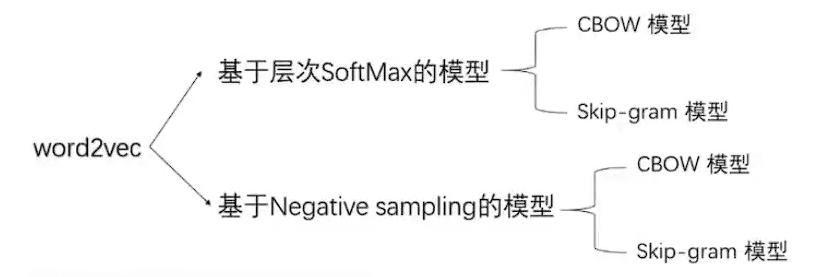
word2vec的两种改进方法：一种是基于Hierarchical Softmax，另一种是基于Negative Sampling。

第三节 Huffman Tree(哈夫曼树)

3.3.1 树的概念

概念	定义
二叉树	每个节点最多有两个子树的树结构
根节点	一棵树最上面的节点
父节点	如果一个节点下面连接多个节点，那么该节点称为父节点
子节点	一个节点含有的子树的根节点称为该节点的子节点
叶子节点	没有任何子节点的节点
节点的度	一个节点拥有的子树数量
树的深度	树中节点的最大层数
父节点/父亲节点	如果一个节点有子节点，则当前节点为子节点的父节点
子节点/孩子节点	与父节点相连的下一层节点为该父节点的子节点
兄弟节点	具有相同父节点的节点互称为兄弟节点

3.3.2 哈夫曼编码算法原理

给定N个权值作为N个叶子结点，构造一棵二叉树，若该树的带权路径长度达到最小，称这样的二叉树为最优二叉树，也称为哈夫曼树(Huffman Tree)。

哈夫曼树是带权路径长度最短的树，权值较大的结点离根较近。

在线动画演示1：https://cmps-people.ok.ubc.ca/ylucet/DS/Huffman.html

在线演示2：https://www.csfieldguide.org.nz/en/interactives/huffman-tree/

参考：https://blog.csdn.net/q1246192888/article/details/106495329

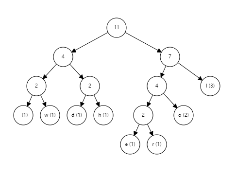
哈夫曼树的构建步骤：

1. 选择与合并：从集合中选择权值最小的两个节点，使用权值最小的两个节点作为左右子树，构造新的树，新的树的权值为左右子树权值之和。使用权值最小的两个节点构建新的树时，应该将权值较小的节点作为左子树，权值较大的节点作为右子树。如果两个节点的权值相同，则将深度较小的作为左子树。
2. 增加与删除：从集合中删除权值最小的两个节点，然后将新创建的节点加入集合。集合中的节点数目减一。减少两个节点，新增一个节点。
3. 重复操作：不断重复上述两个步骤，直到集合中只剩下一个元素为止，即最后哈夫曼树的根节点。

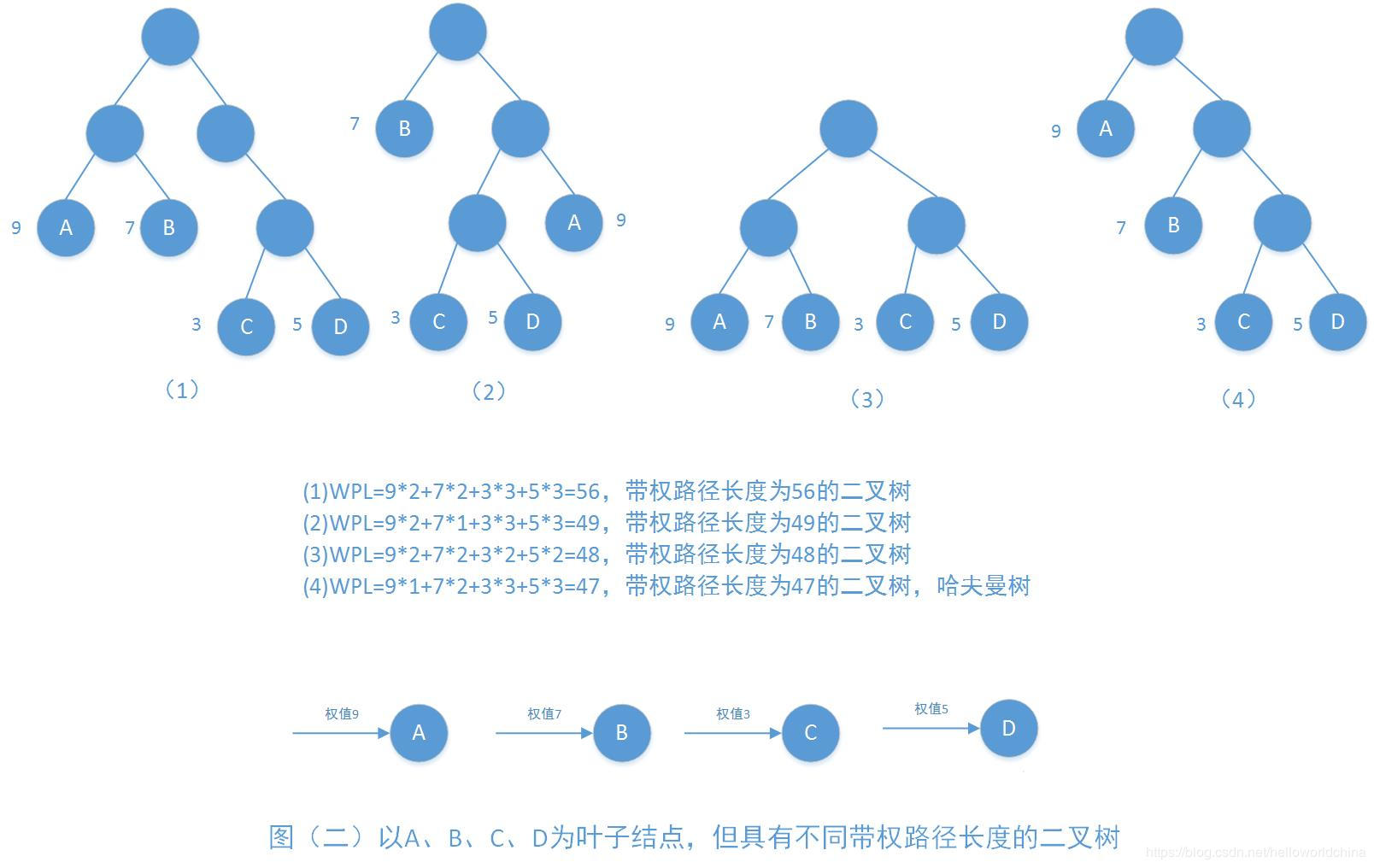
所以（4）的权值最小，因此（4）就是最优哈夫曼树。

分成softmax就是将节点A、B、C、D看成是一个个词，而权重则看成是词出现的次数或频率。

3.3.3 哈夫曼编码的用途

它的主要作用有以下几点：

1. 数据压缩：通过为不同的字符分配不同长度的编码，使得经常出现的字符分配较短的编码，不常出现的字符分配较长的编码，从而实现高效的数据压缩，减少存储空间和传输带宽的需求。
2. 提高传输效率：在数据传输过程中，使用哈夫曼编码可以加快传输速度，降低传输成本。
3. 无损编码：在压缩和解压过程中能保证数据的完整性，不会丢失信息。

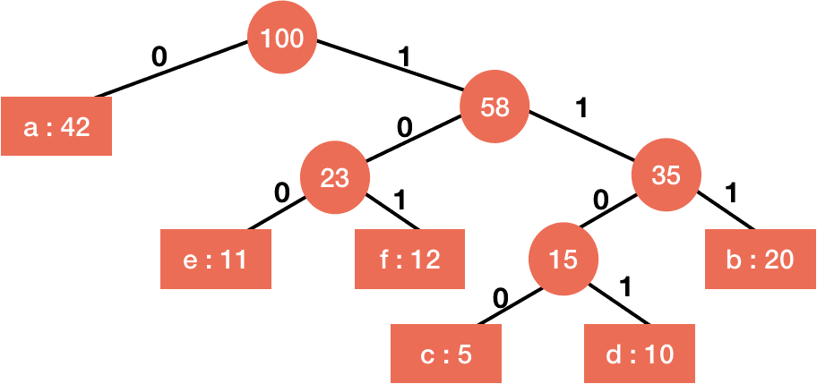
对应编码：

字符	编码
a	0
e	100
f	101
c	1100
d	1101
b	111

假设我要传输 face 这个字符串，以下是ASCII编码与哈夫曼编码的对照。

字符	二进制 ASCII 码	哈夫曼编码
f	01100110	101
a	01100001	0
c	01100011	1100
e	01100101	100

第四节 Hierarchical Softmax (层级Softmax)

3.4.1 Hierarchical Softmax介绍

Hierarchical（读音：海尔洛奇狗）softmax 主要是为了解决 softmax 计算的效率问题。在传统的 softmax 中，需要计算所有词汇的概率分布，这在大规模词汇上会变得非常昂贵，因为 softmax 的计算复杂度与词汇量呈线性关系。

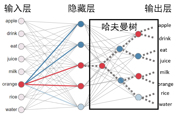
Hierarchical softmax 利用了树结构，将词汇按照概率分布组织成二叉树（通常使用哈夫曼树），从而将整个词汇量的 softmax 分解成多个较小规模的 softmax 计算，极大地降低了计算复杂度。它通过将单词表示为一棵二叉树，每个单词对应二叉树上的一个叶子节点，并从根节点开始递归地计算概率。

在 Word2Vec 模型中，使用哈夫曼树来代替从隐藏层到输出 softmax 层的映射。哈夫曼树的所有内部节点类似于神经网络隐藏层的神经元，其中根节点的词向量对应投影后的词向量，而叶子节点类似于之前神经网络 softmax 输出层的神经元，且叶子节点的个数就是词汇表的大小。

在 Hierarchical softmax 中，Sigmoid 函数用于判别正类和负类，然后这些概率值在树的层次结构中进行传递和组合，最终得到每个单词的概率分布。

在构建哈夫曼树后，规定沿着左子树走为负类（哈夫曼树编码1），沿着右子树走为正类（哈夫曼树编码0）。判别正类和负类的方法是使用 sigmoid 函数，即：

$$ sigmoid(x)=\frac{1}{1+e^{-x}} $$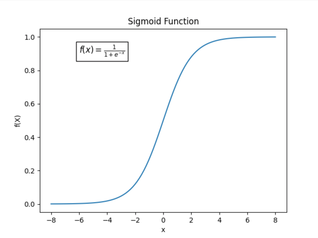

3.4.2 构建Hierarchical Softmax步骤

构建Hierarchical Softmax的过程可以分为以下几个步骤：

1. 构建哈夫曼树（Huffman Tree）：

   • 首先，使用哈夫曼编码构建一个高效的树状结构。哈夫曼树是一种自适应熵编码树，它可以根据词频为词汇表中的每个词分配一个唯一的二进制编码。
   • 具体过程如下：
     • 计算词汇表中每个词的频率。
     • 将每个词视为一个叶子节点，并根据频率将这些节点插入优先队列。
     • 反复从队列中取出两个频率最低的节点，创建一个新的父节点，该父节点的频率是两个子节点频率之和。
     • 将新创建的父节点插入队列中，直到队列中只剩下一个节点，这个节点就是哈夫曼树的根节点。

2. 为每个词分配路径和编码：

   • 在哈夫曼树中，每个词的路径从根节点到叶子节点。路径上的每个节点都包含一个二进制编码（0或1）。
   • 通过遍历哈夫曼树，可以为词汇表中的每个词分配一个唯一的二进制编码（哈夫曼编码）。

3. 计算条件概率：

   • 使用Skip-gram模型的输出来预测上下文词时，可以通过哈夫曼树中的路径来计算条件概率。
   • 给定中心词和目标上下文词，沿着哈夫曼树的路径从根节点到目标词的叶子节点，每个节点对应一个二进制决策（向左或向右）。
   • 条件概率可以通过路径上每个节点的概率乘积来计算。例如，如果路径上的节点决策为向左的概率为( p )，向右的概率为 ( 1 - p )，那么整个路径的概率是这些概率的乘积。

4. 优化目标函数：

   • 使用负对数似然损失函数来优化模型参数。

   • 对于每个中心词和上下文词对，通过沿哈夫曼树的路径计算损失，然后对整个训练语料库中的所有词对进行累加，得到总的损失函数。

   • 使用梯度下降等优化方法来最小化这个损失函数，更新模型参数。

3.4.3 具体例子

3.4.3.1 例子1

假设我们的词汇表是：[“A”, “B”, “C”, “D”]，它们的频率分别是：5, 9, 12, 13。

构建哈夫曼树：

打开网址：https://cmps-people.ok.ubc.ca/ylucet/DS/Huffman.html

输入TEXT：AAAAABBBBBBBBBCCCCCCCCCCCCDDDDDDDDDDDDD

结合步骤查看过程

1. 将所有词插入优先队列，根据频率排序：[“A”, “B”, “C”, “D”]。
2. 取出频率最低的两个词”A”和”B”，创建一个新的父节点，其频率是5 + 9 = 14，将其插入队列中。
3. 现在队列中有三个节点：[14, 12, 13]，取出频率最低的两个词”12”和”13”，创建一个新的父节点，其频率是12 + 13 = 25，将其插入队列中。
4. 现在队列中有两个节点：[14, 25]，取出这两个节点，创建一个新的父节点，其频率是14 + 25 = 39，这个节点是哈夫曼树的根节点。

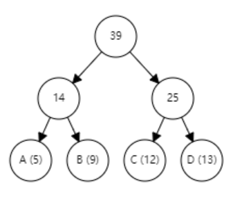
为每个词分配路径和编码：

• “A”的路径是[0, 0]，编码是”00”。
• “B”的路径是[0, 1]，编码是”01”。
• “C”的路径是[1, 0]，编码是”10”。
• “D”的路径是[1, 1]，编码是”11”。

计算条件概率：

• 给定中心词和目标上下文词，通过哈夫曼树的路径计算条件概率。例如，计算 P(“B” | 中心词) 时，沿着路径[0, 1]，计算每个节点上的概率乘积。

具体过程:

节点上的概率计算:

对于每个节点上的二元决策，使用 sigmoid 函数计算概率。假设节点 $n$ 上的向量为 $\theta_n$，中心词的词向量为 $\mathbf{v}_{center}$，那么在节点 $n$ 处：

向左（0）的概率为：

$$ \begin{aligned} P(left|center) &= \sigma(\theta*n \cdot \mathbf{v}*{center}) \\&= \frac{1}{1 + e^{-\theta*n \cdot \mathbf{v}*{center}}} \end{aligned} $$

向右（1）的概率则为：

$$ P(right|center) = 1 - \sigma(\theta*n \cdot \mathbf{v}*{center}) $$

沿路径计算条件概率:

对于词汇 “B”，其路径是 [0, 1]，我们需要沿路径计算每个节点上的概率并取乘积。具体来说：

在根节点到左子节点（0）：

$$ P(\text{left at root}|\text{center}) = \sigma(\theta*{root} \cdot \mathbf{v}*{center}) $$

在左子节点到右子节点（1）：

$$ P(\text{right at left child}|\text{center}) = 1 - \sigma(\theta*{left} \cdot \mathbf{v}*{center}) $$

最终，条件概率 $P(\text{"B"}|\text{center})$ 为：

$$ P(\text{"B"}|\text{center}) = \sigma(\theta*{root} \cdot \mathbf{v}*{center}) \times (1 - \sigma(\theta*{left} \cdot \mathbf{v}*{center})) $$

3.4.3.2 例子2

1. 路径计算：假设要预测词汇 $w$，从根节点到词汇 $w$ 对应的叶子节点的路径为 $(n_0, n_1, \ldots, n_{L-1})$。

2. 节点计算：对于路径上的每个节点 $n_i$，使用模型参数 $\theta_{n_i}$ 和输入向量 $h$ 计算点积，然后通过 sigmoid 函数来计算概率。

   $$ p(n*i) = \sigma(\theta*{n_i} \cdot h) $$

其中，σ 表示 sigmoid 函数，定义为：

$$ \sigma(x) = \frac{1}{1 + e^{-x}} $$

3. 路径概率：整个路径的概率是路径上所有节点概率的乘积或组合。在二叉树的情况下，对于每个节点 $n_i$，我们根据路径选择使用 $p(n_i)$ 或 $1 - p(n_i)$。$$ P(w) = \prod*{i=0}^{L-1} \sigma(\theta*{n*i} \cdot h)^{y_i} (1 - \sigma(\theta*{n_i} \cdot h))^{1 - y_i} $$ 其中， $y_i$ 是路径选择的指示变量，当选择路径上的左子节点时 $y_i = 1$，右子节点时 $y_i = 0$。

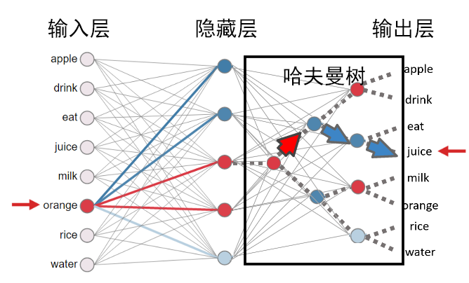
结合下图，尝试一下：

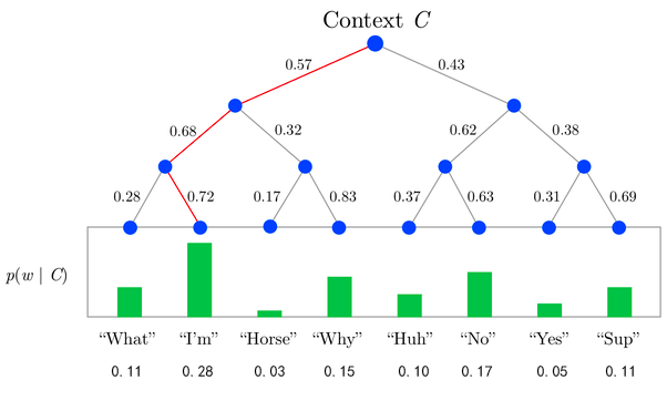
现在需要计算 $“I'm”$的概率，路径上的各节点的概率如下：

• 在根节点选择左边的概率：0.57
• 在左子节点选择左边的概率：0.68
• 在左子节点的左子节点选择右边的概率：0.72

给定中心词的词向量 $h$，每个节点的概率计算如下：

$$ \begin{aligned} P(\text{left at root}|\text{center}) &= 0.57 \\ P(\text{left at left child}|\text{center}) &= 0.68 \\ P(\text{right at left-left child}|\text{center}) &= 0.72 \end{aligned} $$

词汇 $w$ 的路径为：左（0），左（0），右（1）

根据路径，令 $y_i$ 表示选择方向的指示变量，路径中 $y_i = 0$ 表示选择左边，$y_i = 1$ 表示选择右边：

$$ P(w|\text{center}) = \prod*{i=0}^{L-1} \sigma(\theta*{n*i} \cdot h)^{y_i} (1 - \sigma(\theta*{n_i} \cdot h))^{1 - y_i} $$

代入我们的示例：

$$ \begin{aligned} P(w|\text{center}) &= \sigma(\theta*{n_0} \cdot h)^{0} \times (1 - \sigma(\theta*{n*0} \cdot h))^{1-0} \\ & \quad \times \sigma(\theta*{n*1} \cdot h)^{0} \times (1 - \sigma(\theta*{n*1} \cdot h))^{1-0} \\ & \quad \times \sigma(\theta*{n*2} \cdot h)^1 \times (1 - \sigma(\theta*{n_2} \cdot h))^{1-1} \\ \\&= 1 \times 0.57^1 \times 1 \times 0.68^1 \times 0.72^1 \times 1 \\&= 0.57 \times 0.68 \times 0.72 \\&\approx 0.28 \end{aligned} $$

第五节 基于分层Softmax的CBoW模型

基于分层Softmax的CBoW（Continuous Bag of Words）模型是一种用于自然语言处理（NLP）的技术，特别是在词嵌入（word embedding）方面非常有用。

CBoW模型的目标是通过上下文词（context words）预测目标词（target word）。分层Softmax是一种高效的Softmax变体，用于加速训练过程，特别是在处理大规模词汇表时。

3.5.1 基于分层Softmax的优化

Softmax函数在处理大规模词汇表时计算成本很高。分层Softmax（Hierarchical Softmax）通过使用二叉树结构将计算复杂度从$O(V)$（V是词汇表大小）降低到$O(\log V)$。每个词在二叉树中的路径被用作预测目标词的步骤，从而减少了计算量。

3.5.2 目标函数（对数似然）

CBoW模型的目标是最大化目标词的对数似然。给定上下文词$c_1, c_2, \ldots, c_{2m}$，目标是预测中心词$w_o$。模型的目标函数是最大化目标词在上下文中的条件概率：

$$ P(w*o | c_1, c_2, \ldots, c*{2m}) $$

对于整个训练数据集，这个目标可以表示为最大化所有上下文和目标词对的对数似然：

$$ \mathcal{L} = \sum*{t=1}^T \log P(w*{o*t} | c*{t,1}, c*{t,2}, \ldots, c*{t,2m}) $$

在分层Softmax的上下文中，目标词$w_o$的概率被分解为沿着二叉树路径的节点概率的乘积。具体的对数似然表示为：

$$ \log P(w*o | h) = \sum*{n=1}^{L(w_o)} \log P(d_n(w_o) | h) $$

3.5.3 分层Softmax公式

对于给定的上下文词$C$，目标是最大化目标词$w_o$的概率：

$$ P(w*o|C) = \prod*{n=1}^{L(w_o)} P(d_n(w_o)|C) $$

其中，$L(w_o)$是词$w_o$在二叉树中的路径长度，$d_n(w_o)$是第$n$步的二进制决策。

具体的概率计算为：

$$ P(d*n(w_o)=1|C) = \sigma(v*{d_n(w_o)}^\top h) $$ $$ P(d*n(w_o)=0|C) = 1 - \sigma(v*{d_n(w_o)}^\top h) $$

其中，$\sigma(x)$是Sigmoid函数，$v_{d_n(w_o)}$是二叉树中第$n$个节点的向量，$h$是上下文词向量的平均值。

3.5.4 计算例子

分层Softmax通过构建二叉树来表示词汇表中的每个词。假设词汇表中的词通过一个二叉树结构组织起来。对于每个词，我们定义其在二叉树中的路径。例如：

      (root)
      /    \
    (1)    (2)
   /  \    /  \
(3)  (4) (5)  (6)
the quick brown fox

在这个树中，每个词的路径如下：

• "the": (root) -> (1) -> (3)
• "quick": (root) -> (1) -> (4)
• "brown": (root) -> (2) -> (5)
• "fox": (root) -> (2) -> (6)

为了预测词$w_o$，我们沿着其路径计算每个节点的二进制决策概率。具体来说：

对于给定的上下文词$C$，目标是最大化目标词$w_o$的概率：

$$ P(w*o|C) = \prod*{n=1}^{L(w_o)} P(d_n(w_o)|C) $$

其中，$L(w_o)$是词$w_o$在二叉树中的路径长度，$d_n(w_o)$是第$n$步的二进制决策。具体的概率计算为：

$$ P(d*n(w_o)=1|C) = \sigma(v*{d_n(w_o)}^\top h) $$ $$ P(d*n(w_o)=0|C) = 1 - \sigma(v*{d_n(w_o)}^\top h) $$

其中，$\sigma(x)$是Sigmoid函数，$v_{d_n(w_o)}$是二叉树中第$n$个节点的向量，$h$是上下文词向量的平均值。

具体例子：

假设我们有一个简单的句子：”the quick brown fox jumps over the lazy dog”。

我们选取一个上下文窗口大小为2，例如，对目标词”fox”，其上下文词为[“the”, “quick”, “brown”, “jumps”]。

1. 构建上下文向量：假设词向量$\mathbf{v}_{\text{the}}$、$\mathbf{v}_{\text{quick}}$、$\mathbf{v}_{\text{brown}}$和$\mathbf{v}_{\text{jumps}}$分别为：

$$ \begin{aligned} \mathbf{v}_{\text{the}} &= [0.2, 0.1, 0.3] \\\mathbf{v}_{\text{quick}} &= [0.4, 0.3, 0.5] \\\mathbf{v}_{\text{brown}} &= [0.1, 0.4, 0.3] \\\mathbf{v}_{\text{jumps}} &= [0.3, 0.2, 0.4] \end{aligned} $$

上下文向量$h$为：

$$ \begin{aligned} h &= \frac{1}{4} (\mathbf{v}_{\text{the}} + \mathbf{v}_{\text{quick}} + \mathbf{v}_{\text{brown}} + \mathbf{v}_{\text{jumps}}) \\&= \frac{1}{4} ([0.2, 0.1, 0.3] + [0.4, 0.3, 0.5] + [0.1, 0.4, 0.3] + [0.3, 0.2, 0.4]) \\&= \frac{1}{4} ([1.0, 1.0, 1.5]) \\&= [0.25, 0.25, 0.375] \end{aligned} $$

2. 计算路径概率：假设”fox”的路径为 (root) -> (2) -> (6)，且$\mathbf{v}_{\text{(2)}} = [0.5, 0.4, 0.3]$，$\mathbf{v}_{\text{(6)}} = [0.6, 0.7, 0.8]$。

• 第一步：(root) -> (2)

$$ \begin{aligned} \mathbf{v}\_{\text{(2)}}^\top h &= [0.5, 0.4, 0.3] \cdot [0.25, 0.25, 0.375] \\&= 0.5 \times 0.25 + 0.4 \times 0.25 + 0.3 \times 0.375 \\&= 0.125 + 0.1 + 0.1125 \\&= 0.3375 \end{aligned} $$ $$ \begin{aligned} P(d*1(\text{fox}) = 1|C) &= \sigma(\mathbf{v}*{\text{(2)}}^\top h) \\&= \sigma(0.3375) \\&= \frac{1}{1 + e^{-0.3375}} \\&\approx 0.5836 \end{aligned} $$

• 第二步：(2) -> (6)

$$ \begin{aligned} \mathbf{v}\_{\text{(6)}}^\top h &= [0.6, 0.7, 0.8] \cdot [0.25, 0.25, 0.375] \\&= 0.6 \times 0.25 + 0.7 \times 0.25 + 0.8 \times 0.375 \\&= 0.15 + 0.175 + 0.3 \\&= 0.625 \end{aligned} $$ $$ \begin{aligned} P(d*2(\text{fox}) = 0|C) &= 1 - \sigma(\mathbf{v}*{\text{(6)}}^\top h) \\&= 1 - \sigma(0.625) \\&= 1 - \frac{1}{1 + e^{-0.625}} \\&\approx 1 - 0.6514 \\&= 0.3486 \end{aligned} $$

3. 计算总概率：

$$ \begin{aligned} P(\text{fox}|C) &= P(d_1(\text{fox}) = 1|C) \times P(d_2(\text{fox}) = 0|C) \\&= 0.5836 \times 0.3486 \\&\approx 0.2034 \end{aligned} $$

4. 计算对数似然：

$$ \begin{aligned} \log P(\text{fox}|C) &= \log P(d_1(\text{fox}) = 1|C) + \log P(d_2(\text{fox}) = 0|C) \\&= \log 0.5836 + \log 0.3486 \\&\approx -0.5376 + (-1.0548) \\&= -1.5924 \end{aligned} $$

5. 更新梯度

   在 CBoW 模型中，我们的主要参数是词向量 $\mathbf{v}$。我们的目标是通过最大化对数似然函数来更新这些参数。

   首先，我们需要计算对数似然函数关于参数的梯度。然后，我们可以使用梯度下降算法来更新参数。

   在我们的具体例子中，我们将以 “fox” 作为目标词为例来更新参数。假设我们已经计算了 $P(\text{fox}|C)$ 和 $\log P(\text{fox}|C)$，并且我们已经计算了上下文向量 $\mathbf{h}$ 以及路径概率 $P(d_1(\text{fox})=1|C)$ 和 $P(d_2(\text{fox})=0|C)$。

   现在，我们来计算对数似然函数关于目标词 “fox” 的词向量 $\mathbf{v}_{\text{fox}}$ 的梯度：

$$ \frac{\partial \log P(\text{fox}|C)}{\partial \mathbf{v}\_{\text{fox}}} = \left(1 - P(d_1(\text{fox})=1|C)\right) \cdot \mathbf{h} $$

在我们的例子中，$P(d_1(\text{fox})=1|C) \approx 0.5836$，因此：

$$ \begin{aligned} \frac{\partial \log P(\text{fox}|C)}{\partial \mathbf{v}\_{\text{fox}}} &= (1 - 0.5836) \cdot \mathbf{h} \\&\approx 0.4164 \cdot [0.25, 0.25, 0.375] \\&= [0.1041, 0.1041, 0.1562] \end{aligned} $$

现在，我们可以使用梯度下降算法来更新 $\mathbf{v}_{\text{fox}}$。假设我们选择一个学习率 $\eta = 0.1$，更新规则如下：

$$ \mathbf{v}_{\text{fox}}^{(t+1)} = \mathbf{v}_{\text{fox}}^{(t)} - \eta \cdot \frac{\partial \log P(\text{fox}|C)}{\partial \mathbf{v}\_{\text{fox}}} $$

假设初始的 $\mathbf{v}_{\text{fox}}^{(0)} = [0.3, 0.4, 0.5]$，那么更新后的 $\mathbf{v}_{\text{fox}}^{(1)}$ 为：

$$ \begin{aligned} \mathbf{v}\_{\text{fox}}^{(1)} &= [0.3, 0.4, 0.5] - 0.1 \cdot [0.1041, 0.1041, 0.1562] \\&\approx [0.3, 0.4, 0.5] - [0.01041, 0.01041, 0.01562] \\&\approx [0.28959, 0.38959, 0.48438] \end{aligned} $$

这样，我们就完成了一次参数更新。接下来，我们可以使用更新后的参数重新计算路径概率，并继续进行更多的迭代更新，直到达到停止条件为止。

通过具体的数值计算，可以直观地理解分层Softmax在CBoW模型中的应用及其数学原理。这种计算方法极大地提高了在大规模词汇表上的计算效率。

3.5.5 代码实现

下面是一个基于PyTorch实现的简化版CBoW模型，结合分层Softmax：

import torch
import torch.nn as nn
import torch.optim as optim

class CBOWModel(nn.Module):
    def __init__(self, vocab_size, embedding_dim, tree_structure):
        super(CBOWModel, self).__init__()
        self.embeddings = nn.Embedding(vocab_size, embedding_dim)
        self.tree_structure = tree_structure
        self.embedding_dim = embedding_dim

    def forward(self, context_word_indices, target_word_index):
        context_embeddings = self.embeddings(context_word_indices)
        context_embedding_mean = torch.mean(context_embeddings, dim=0)
        target_path = self.tree_structure[target_word_index]

        log_prob = 0
        for node, direction in target_path:
            node_vector = self.embeddings(node)
            prob = torch.sigmoid(torch.dot(node_vector, context_embedding_mean))
            log_prob += torch.log(prob if direction == 1 else (1 - prob))

        return log_prob

# 树结构示例（简单示例，每个单词在树中的路径）
tree_structure = {
    0: [(1, 1), (2, 0)],
    1: [(1, 1), (3, 1)],
    2: [(4, 0)],
    3: [(4, 1)]
}

# 参数
vocab_size = 5
embedding_dim = 10

# 模型初始化
model = CBOWModel(vocab_size, embedding_dim, tree_structure)
optimizer = optim.SGD(model.parameters(), lr=0.01)

# 示例训练步骤
context_word_indices = torch.tensor([0, 1, 2], dtype=torch.long)
target_word_index = torch.tensor(3, dtype=torch.long)

# 前向传播
log_prob = model(context_word_indices, target_word_index)

# 计算损失
loss = -log_prob
loss.backward()
optimizer.step()

print("Training step completed with loss:", loss.item())

第六节 基于分层Softmax的Skip-gram模型

基于分层Softmax的Skip-gram模型是一种用于自然语言处理中词向量学习的模型。Skip-gram模型的目标是学习一个词向量空间，在这个空间中，相似的词被映射到彼此附近的位置。分层Softmax是一种用于处理输出层的技术，它通过构建一个多层次的树状结构来提高训练效率。

在传统的Skip-gram模型中，输出层通常是一个大的softmax层，它需要对所有词汇进行计算，这会导致训练速度变慢，特别是在大规模语料库上。为了解决这个问题，分层Softmax被引入。

分层Softmax使用树状结构将词汇划分为不同的类别，每个词汇都被赋予一个路径，而路径上的节点则对应于不同的词汇。这样，输出层的计算可以通过沿着这个树状结构进行，而不需要对所有词汇进行计算。这种方法可以显著减少计算量，提高训练速度。

3.6.1 目标函数

基于分层Softmax的Skip-gram模型的目标函数通常使用负对数似然损失函数来定义。在这个模型中，给定一个中心词，我们的目标是最大化上下文词的条件概率。假设我们有一个长度为T的训练序列，其中每个词被表示为一个one-hot向量。假设中心词是c，上下文词是o，那么目标函数可以表示为：

$$ J(\theta) = -\frac{1}{T} \sum*{t=1}^{T} \sum*{-m \leq j \leq m, j \neq 0} \log P(o_t | c_t; \theta) $$

其中，$P(o_t | c_t; \theta)$ 是给定中心词 $c_t$ 情况下上下文词 $o_t$ 的条件概率，$\theta$ 是模型参数，$m$ 是上下文窗口大小。
​
基于分层Softmax的Skip-gram模型使用了分层Softmax技术来估计条件概率。具体来说，它使用了一个多层次的树状结构，其中每个词被分配到树中的一个节点。通过从根节点开始，沿着路径移动到达目标词所在的叶子节点，可以计算条件概率。这样的话，目标函数可以重新写成：

$$ J(\theta) = -\frac{1}{T} \sum*{t=1}^{T} \sum*{-m \leq j \leq m, j \neq 0} \sum*{i=1}^{L(w)} \log P(w*{t+j} = w_i | c_t; \theta) $$

其中，$w_i$ 是第i个词，$L(w)$ 是词汇表的大小，$P(w_{t+j} = w_i | c_t; \theta)$ 是给定中心词 $c_t$ 情况下，上下文词 $w_{t+j}$ 是第 $i$ 个词的条件概率。

3.6.2 计算例子

假设我们有以下句子：

1. “The quick brown fox jumps over the lazy dog”
2. “A cat is chasing a mouse”
3. “The sun sets in the west”
4. “Birds fly in the sky”

我们的词汇表包括：[“The”, “quick”, “brown”, “fox”, “jumps”, “over”, “lazy”, “dog”, “A”, “cat”, “is”, “chasing”, “mouse”, “sun”, “sets”, “in”, “west”, “Birds”, “fly”, “sky”]

现在，让我们选择一个中心词和一个上下文词来计算条件概率。

假设我们选择中心词是”The”，上下文词是”quick”。

我们的目标是计算

$$ P(\text{"quick"}|\text{"The"}) $$

我们需要遍历词汇表中的每个词，并查看它们在分层Softmax树中的路径，以计算条件概率。假设在我们的分层Softmax树中，”quick”的路径是[0, 1, 2, 7]，而”The”的路径是[0, 3, 5]。

我们需要计算路径上每个节点的概率，并将它们相乘以获得最终的条件概率。

$$ \begin{aligned} P(\text{"quick"}|\text{"The"}) &= P(\text{"quick"}| \text{"The"}; \theta) \\&= P(\text{"quick"}| \text{"The"}) \times P(\text{"quick"}| \text{"The"}, \text{"brown"}) \times P(\text{"quick"}| \text{"The"}, \text{"brown"}, \text{"fox"}) \end{aligned} $$

然后，我们根据树状结构中每个节点的概率，计算路径上的条件概率。最后，将它们相乘得到最终的条件概率。

希望这个完整的计算示例能够帮助你更好地理解基于分层Softmax的Skip-gram模型的计算过程。

第七节 什么是负采样（Negative Sampling）

Negative Sampling（简称 NEG）是 Tomas Mikolov 等人提出的，它是 Noise Contrastive Estimation（NCE）的一个简化版本，目的是用来提高训练速度并改善所得词向量的质量。与 Hierarchical Softmax 相比，NEG 不再使用复杂的 Hufman 树，而是利用相对简单的随机负采样，能大幅度提高性能，因而可作为 Hierarchical Softmax 的一种替代。

负采样是一种优化技术，用于替代传统的softmax，减少计算开销。在训练过程中，对于每个正样本（中心词和上下文词对），我们随机选择一些负样本，这些负样本是与当前上下文无关的词。模型的目标是使得正样本的点积尽可能大，而负样本的点积尽可能小。

Negative Sampling 是一种在训练词嵌入（如 Word2Vec）时常用的技巧，它能有效地加速训练过程并提高嵌入的质量。以下是 Negative Sampling 的详细过程，包括其背景、数学描述和代码实现。

Negative Sampling 通过仅对一小部分“负样本”而不是整个词汇表进行计算，大大减小了计算量。

3.7.1 数学描述

假设我们有一个中心词 ( w ) 和其上下文词 ( c )，我们的目标是最大化以下目标函数：

$$ \log \sigma (v*c^\top v_w) + \sum*{i=1}^k \mathbb{E}_{w_i \sim P_n(w)} [\log \sigma (-v_{w_i}^\top v_w)] $$

其中：

• $\sigma(x)$ 是 sigmoid 函数。
• $v_c$ 是上下文词 $c$ 的词嵌入向量。
• $v_w$ 是中心词 $w$ 的词嵌入向量。
• $P_n(w)$ 是负样本分布（通常是词频分布的某种变形）。
• $k$ 是负样本的数量。
• $w_i$ 是从负样本分布中抽取的负样本。

$\mathbb{E}$ 在数学中读作 “E”。具体来说，$\mathbb{E}$ 是期望值（或期望、均值）的符号，常用于概率论和统计学中，表示一个随机变量的平均值或期望值。

$\mathbb{E}_{w_i \sim P_n(w)}$ 表示从负样本分布 $P_n(w)$ 中抽取负样本并计算它们的期望值。通常，这个期望值通过从分布中随机抽取若干负样本来近似。

期望值在概率论和统计学中是一个重要概念。简单来说，期望值是对随机变量可能取值的一种加权平均。它是通过将每个可能的取值乘以其对应的概率，再将所有结果相加得到的。期望值反映了在大量重复试验中，该随机变量的平均预期取值。

例如，对于一个投掷骰子的试验，骰子每个面出现的概率均为 1/6，那么骰子点数的期望值就是(1×1/6 + 2×1/6 + 3×1/6 + 4×1/6 + 5×1/6 + 6×1/6) = 3.5，表示多次投掷后平均预期得到的点数大致是 3.5。

期望值在决策分析、风险评估、经济预测等许多领域都有广泛应用。

过程

1. 正样本计算：

   • 计算中心词和真实上下文词的相似度，并应用 sigmoid 函数。

2. 负样本选择：

   • 根据某种负样本分布（如词频分布的某种变形），随机选择 $k$ 个负样本。

3. 负样本计算：

   • 计算中心词和负样本的相似度，并应用负的 sigmoid 函数。

4. 更新：

   • 根据正样本和负样本的计算结果，更新词嵌入矩阵。

3.7.2 具体例子说明

假设我们有一个小词汇表和简单的嵌入矩阵如下：

• 词汇表：['I', 'love', 'machine', 'learning', 'and', 'AI']
• 词汇表大小：6
• 嵌入维度：2
• 嵌入矩阵：

  I           -> [0.1, 0.2]
  love        -> [0.3, 0.4]
  machine     -> [0.5, 0.6]
  learning    -> [0.7, 0.8]
  and         -> [0.9, 1.0]
  AI          -> [1.1, 1.2]

我们以词对 (‘love’, ‘machine’) 作为正样本，并从负样本分布中随机选取 2 个负样本，假设选到的负样本为 ‘I’ 和 ‘and’。

计算步骤：

1. 正样本计算：

   • 中心词 ‘love’ 的嵌入向量 $v_w = [0.3, 0.4]$
   • 上下文词 ‘machine’ 的嵌入向量 $v_c = [0.5, 0.6]$
   • 点积 $v_c^\top v_w = 0.3 \cdot 0.5 + 0.4 \cdot 0.6 = 0.15 + 0.24 = 0.39$
   • $\sigma(v_c^\top v_w) = \sigma(0.39) \approx 0.596$ （这里假设 sigmoid 函数的计算结果）
   • 正样本损失 $-\log(\sigma(0.39)) \approx -\log(0.596) \approx 0.517$

2. 负样本计算：

   • 负样本 ‘I’ 的嵌入向量 $v_{w_i1} = [0.1, 0.2]$
     • 点积 $v_{w_i1}^\top v_w = 0.1 \cdot 0.3 + 0.2 \cdot 0.4 = 0.03 + 0.08 = 0.11$
     • $\sigma(-v_{w_i1}^\top v_w) = \sigma(-0.11) \approx 0.473$
     • 损失 $-\log(\sigma(-0.11)) \approx -\log(0.473) \approx 0.749$
   • 负样本 ‘and’ 的嵌入向量 $v_{w_i2} = [0.9, 1.0]$
     • 点积 $v_{w_i2}^\top v_w = 0.9 \cdot 0.3 + 1.0 \cdot 0.4 = 0.27 + 0.4 = 0.67$
     • $\sigma(-v_{w_i2}^\top v_w) = \sigma(-0.67) \approx 0.339$
     • 损失 $-\log(\sigma(-0.67)) \approx -\log(0.339) \approx 1.082$

3. 总负样本损失：

   • $0.749 + 1.082 = 1.831$

4. 总损失：

   • 正样本损失 $0.517$ 加上总负样本损失 $1.831$
   • 总损失 $0.517 + 1.831 = 2.348$

3.7.3 代码实现

import torch
import torch.nn as nn
import torch.optim as optim

# 设置词汇表大小和嵌入维度
vocab_size = 6
embedding_dim = 2

# 创建嵌入层，并手动设置嵌入矩阵
embedding = nn.Embedding(vocab_size, embedding_dim)
embedding.weight.data = torch.tensor([
    [0.1, 0.2],  # I
    [0.3, 0.4],  # love
    [0.5, 0.6],  # machine
    [0.7, 0.8],  # learning
    [0.9, 1.0],  # and
    [1.1, 1.2]   # AI
])

# 定义 sigmoid 函数
sigmoid = nn.Sigmoid()

# 中心词和上下文词的索引
center_word_idx = torch.tensor([1])  # love
context_word_idx = torch.tensor([2])  # machine

# 正样本计算
center_embed = embedding(center_word_idx)  # shape: (1, embedding_dim)
context_embed = embedding(context_word_idx)  # shape: (1, embedding_dim)

# 计算正样本的相似度并应用 sigmoid
positive_score = sigmoid(torch.dot(center_embed, context_embed.t()))
positive_loss = -torch.log(positive_score)

# 负样本选择
negative_sample_indices = torch.tensor([0, 4])  # I, and

# 负样本计算
negative_embed = embedding(negative_sample_indices)  # shape: (num_negative_samples, embedding_dim)

# 计算负样本的相似度并应用负的 sigmoid
negative_scores = sigmoid(-torch.matmul(negative_embed, center_embed.t()))
negative_loss = -torch.sum(torch.log(negative_scores))

# 总损失
loss = positive_loss + negative_loss

print(f"Positive loss: {positive_loss.item()}")
print(f"Negative loss: {negative_loss.item()}")
print(f"Total loss: {loss.item()}")

输出：

Positive loss: 0.5171933174133301
Negative loss: 1.8312934637069702
Total loss: 2.34848690032959

1. Positive loss: 这是正样本的损失，即中心词 ‘love’ 和上下文词 ‘machine’ 的损失，值为 0.517。
2. Negative loss: 这是负样本的总损失，即中心词 ‘love’ 与负样本 ‘I’ 和 ‘and’ 的总损失，值为 1.831。
3. Total loss: 总损失是正样本损失和负样本损失的总和，值为 2.348。

通过这个具体例子，我们展示了如何计算正样本和负样本的损失，并如何在代码中实现这些计算步骤。这样可以更直观地理解 Negative Sampling 的过程。

第八节 基于Negative Sampling的CBoW模型

基于Negative Sampling的Continuous Bag of Words（CBoW）模型是一种高效的词嵌入方法。与传统的CBoW模型相比，负采样显著减少了计算开销，提高了训练速度。下面是基于Negative Sampling的CBoW模型的详细介绍。

3.8.1 算法过程

1. 输入上下文词：对于每个中心词，确定其前后上下文词。例如，给定上下文窗口大小为 $k$，则对于中心词 $w_t$，上下文词为 $[w_{t-k}, ..., w_{t-1}, w_{t+1}, ..., w_{t+k}]$。

2. 上下文词向量求和：将上下文词的词向量进行平均或求和，得到一个上下文向量。

3. 预测中心词：使用上下文向量来预测中心词。这里使用一个二分类器来判断给定的中心词是否是正样本。

4. 负样本选择：随机选择若干负样本，这些负样本是从词汇表中采样得到的，且不在当前上下文中。

5. 目标函数：最大化对正样本的预测概率，同时最小化对负样本的预测概率。具体来说，目标函数为：

   $$ \log \sigma (\vec{v}_{w_O} \cdot \vec{v}_{w*I}) + \sum*{w*k \in \text{neg samples}} \log \sigma (-\vec{v}*{w*k} \cdot \vec{v}*{w_I}) $$

   其中，$\sigma$ 是sigmoid函数，$\vec{v}_{w_O}$ 是中心词向量，$\vec{v}_{w_I}$ 是上下文向量，$\vec{v}_{w_k}$ 是负样本向量。

6. 参数更新：通过反向传播和梯度下降来更新词向量，使得模型能够更准确地预测中心词和区分负样本。

3.8.2 代码示例

以下是一个简单的基于负采样的CBoW模型的实现（使用PyTorch）：

import torch
import torch.nn as nn
import torch.optim as optim
from collections import Counter
import numpy as np

class CBoWNegativeSampling(nn.Module):
    def __init__(self, vocab_size, embedding_dim):
        super(CBoWNegativeSampling, self).__init__()
        self.embeddings = nn.Embedding(vocab_size, embedding_dim)
        self.linear = nn.Linear(embedding_dim, vocab_size)

    def forward(self, context_words):
        embeds = self.embeddings(context_words)
        context_embeds = torch.mean(embeds, dim=0).view(1, -1)
        out = self.linear(context_embeds)
        return out

def train(model, data, word_to_idx, idx_to_word, window_size, num_epochs, learning_rate):
    loss_fn = nn.CrossEntropyLoss()
    optimizer = optim.SGD(model.parameters(), lr=learning_rate)

    for epoch in range(num_epochs):
        total_loss = 0
        for context, target in data:
            context_idxs = torch.tensor([word_to_idx[w] for w in context], dtype=torch.long)
            target_idx = torch.tensor([word_to_idx[target]], dtype=torch.long)

            model.zero_grad()
            log_probs = model(context_idxs)
            loss = loss_fn(log_probs, target_idx)
            loss.backward()
            optimizer.step()

            total_loss += loss.item()
        print(f'Epoch {epoch+1}, Loss: {total_loss}')

# 构建词汇表
sentences = [['the', 'quick', 'brown', 'fox', 'jumps', 'over', 'the', 'lazy', 'dog']]
vocab = set(sum(sentences, []))
word_to_idx = {word: i for i, word in enumerate(vocab)}
idx_to_word = {i: word for i, word in enumerate(vocab)}

# 构建训练数据
data = []
window_size = 2
for sentence in sentences:
    for i, word in enumerate(sentence):
        context = [
            sentence[j]
            for j in range(i - window_size, i + window_size + 1)
            if j != i and j >= 0 and j < len(sentence)
        ]
        target = word
        data.append((context, target))

# 训练模型
embedding_dim = 10
model = CBoWNegativeSampling(len(vocab), embedding_dim)
train(model, data, word_to_idx, idx_to_word, window_size, num_epochs=100, learning_rate=0.01)

推理：

import torch

# 假设我们有一个训练好的模型 model
# 定义一些参数
embedding_dim = 10  # 嵌入维度
vocab_size = len(word_to_idx)  # 词汇表大小

# 创建模型实例并加载预训练的权重（如果有）
model = CBoWNegativeSampling(vocab_size, embedding_dim)
# 如果你有保存的模型权重文件，例如 model.pth
# model.load_state_dict(torch.load('model.pth'))
# model.eval()  # 切换到评估模式

# 定义要推理的上下文词
context_words = ['fox', 'over']
context_idxs = torch.tensor([word_to_idx[word] for word in context_words], dtype=torch.long)

# 进行推理
with torch.no_grad():
    output = model(context_idxs)
    predicted_idx = torch.argmax(output, dim=1).item()

# 输出预测的中心词
predicted_word = idx_to_word[predicted_idx]
print(f'Predicted center word: {predicted_word}')

第九节 基于Negative Sampling的Skip-gram模型

基于Negative Sampling的Skip-gram模型是另一种常用的词嵌入方法，与CBoW模型相比，它通过中心词来预测上下文词。负采样技术在Skip-gram模型中的应用，使得训练过程更加高效。以下是基于Negative Sampling的Skip-gram模型的详细介绍。

3.9.1 算法过程

1. 输入中心词：选定一个中心词 $w_t$。

2. 选择上下文词：确定该中心词的上下文窗口，假设窗口大小为 $k$，则上下文词为 $[w_{t-k}, ..., w_{t-1}, w_{t+1}, ..., w_{t+k}]$。

3. 采样负样本：随机选择若干负样本，这些负样本是从词汇表中采样得到的，且不在当前上下文中。

4. 目标函数：最大化对正样本的预测概率，同时最小化对负样本的预测概率。目标函数为：

   $$ \sum*{w_c \in \text{context}} \left( \log \sigma (\vec{v}*{w*c} \cdot \vec{v}*{w*t}) + \sum*{w*k \in \text{neg samples}} \log \sigma (-\vec{v}*{w*k} \cdot \vec{v}*{w_t}) \right) $$

   其中，$\sigma$ 是sigmoid函数，$\vec{v}_{w_c}$ 是上下文词向量，$\vec{v}_{w_t}$ 是中心词向量，$\vec{v}_{w_k}$ 是负样本向量。

5. 参数更新：通过反向传播和梯度下降来更新词向量，使得模型能够更准确地预测上下文词和区分负样本。

3.9.2 代码示例

以下是一个简单的基于负采样的Skip-gram模型的实现（使用PyTorch）：

import torch
import torch.nn as nn
import torch.optim as optim
import numpy as np
from collections import Counter
import random

class SkipGramNegativeSampling(nn.Module):
    def __init__(self, vocab_size, embedding_dim):
        super(SkipGramNegativeSampling, self).__init__()
        self.in_embeddings = nn.Embedding(vocab_size, embedding_dim)
        self.out_embeddings = nn.Embedding(vocab_size, embedding_dim)

    def forward(self, center_word, context_words, negative_samples):
        center_embed = self.in_embeddings(center_word).unsqueeze(0)
        context_embeds = self.out_embeddings(context_words)
        neg_embeds = self.out_embeddings(negative_samples)

        pos_dot_products = torch.bmm(context_embeds, center_embed.unsqueeze(2)).squeeze()
        neg_dot_products = torch.bmm(neg_embeds, center_embed.unsqueeze(2)).squeeze()

        log_pos = torch.log(torch.sigmoid(pos_dot_products)).sum()
        log_neg = torch.log(torch.sigmoid(-neg_dot_products)).sum()

        loss = -(log_pos + log_neg)
        return loss

def generate_negative_samples(word_to_idx, num_neg_samples, exclude):
    vocab_size = len(word_to_idx)
    negative_samples = []
    while len(negative_samples) < num_neg_samples:
        sample = random.randint(0, vocab_size - 1)
        if sample not in exclude:
            negative_samples.append(sample)
    return torch.tensor(negative_samples, dtype=torch.long)

def train(model, data, word_to_idx, idx_to_word, window_size, num_neg_samples, num_epochs, learning_rate):
    optimizer = optim.SGD(model.parameters(), lr=learning_rate)

    for epoch in range(num_epochs):
        total_loss = 0
        for center, context in data:
            center_idx = torch.tensor([word_to_idx[center]], dtype=torch.long)
            context_idxs = torch.tensor([word_to_idx[w] for w in context], dtype=torch.long)
            negative_samples = generate_negative_samples(word_to_idx, num_neg_samples, set(context_idxs.tolist()))

            model.zero_grad()
            loss = model(center_idx, context_idxs, negative_samples)
            loss.backward()
            optimizer.step()

            total_loss += loss.item()
        print(f'Epoch {epoch+1}, Loss: {total_loss}')

# 构建词汇表
sentences = [['the', 'quick', 'brown', 'fox', 'jumps', 'over', 'the', 'lazy', 'dog']]
vocab = set(sum(sentences, []))
word_to_idx = {word: i for i, word in enumerate(vocab)}
idx_to_word = {i: word for i, word in enumerate(vocab)}

# 构建训练数据
data = []
window_size = 2
for sentence in sentences:
    for i, word in enumerate(sentence):
        context = [
            sentence[j]
            for j in range(i - window_size, i + window_size + 1)
            if j != i and j >= 0 and j < len(sentence)
        ]
        data.append((word, context))

# 训练模型
embedding_dim = 10
num_neg_samples = 5
model = SkipGramNegativeSampling(len(vocab), embedding_dim)
train(model, data, word_to_idx, idx_to_word, window_size, num_neg_samples, num_epochs=100, learning_rate=0.01)

推理：

import torch

# 假设我们有一个训练好的模型 model
# 定义一些参数
embedding_dim = 10  # 嵌入维度
vocab_size = len(word_to_idx)  # 词汇表大小

# 创建模型实例并加载预训练的权重（如果有）
model = CBoWNegativeSampling(vocab_size, embedding_dim)
# 如果你有保存的模型权重文件，例如 model.pth
# model.load_state_dict(torch.load('model.pth'))
# model.eval()  # 切换到评估模式

# 定义要推理的上下文词
context_words = ['fox', 'over']
context_idxs = torch.tensor([word_to_idx[word] for word in context_words], dtype=torch.long)

# 进行推理
with torch.no_grad():
    output = model(context_idxs)
    predicted_idx = torch.argmax(output, dim=1).item()

# 输出预测的中心词
predicted_word = idx_to_word[predicted_idx]
print(f'Predicted center word: {predicted_word}')

阅读扩展

第一节 隐藏层与投影层的区别

让我们通过具体例子来详细说明投影层和隐藏层的区别，包括数学计算和代码实现。

投影层

投影层是人工神经网络中输入层和隐藏层之间的一层。它的作用是将输入数据进行预处理和特征提取，将高维数据映射到低维空间，以便后续的隐藏层进行处理。投影层通常使用线性变换或卷积操作来实现。它的主要目的是降维或将离散输入（如单词的索引）转换为连续的、密集的向量表示。

投影层通常是一个查找表（lookup table），如一个嵌入矩阵 $E \in \mathbb{R}^{V \times d}$，其中 $V$ 是词汇表的大小，$d$ 是嵌入维度。

对于输入的单词索引 $i$，投影层直接返回嵌入矩阵 $E$ 的第 $i$ 行，即$E[i]$。

数学计算

假设我们有一个词汇表大小为 5 的词汇表，包含单词 [“I”, “like”, “to”, “eat”, “apples”]。我们希望将这些单词映射到 3 维的嵌入空间。

嵌入矩阵 $E \in \mathbb{R}^{5 \times 3}$ 可能如下：

$$ E = \begin{bmatrix} 0.1 & 0.3 & 0.5 \\ 0.2 & 0.4 & 0.6 \\ 0.3 & 0.5 & 0.7 \\ 0.4 & 0.6 & 0.8 \\ 0.5 & 0.7 & 0.9 \end{bmatrix} $$ $\mathbb{R}$ 通常读作“实数集（Real number set）”

假设输入单词 “like” 对应索引为 1，则投影层的输出为：

$$ E[1] = \begin{bmatrix} 0.2 & 0.4 & 0.6 \end{bmatrix} $$

代码实现

import torch
import torch.nn as nn

# 假设词汇表大小为 5，嵌入维度为 3
vocab_size = 5
embedding_dim = 3

# 定义嵌入层
embedding_layer = nn.Embedding(vocab_size, embedding_dim)

# 查看嵌入矩阵
print("Embedding matrix:")
print(embedding_layer.weight.data)

# 输入单词的索引
word_index = torch.tensor([1])

# 通过嵌入层查找对应的嵌入向量
embedding_vector = embedding_layer(word_index)
print("\nEmbedding vector for index 1:")
print(embedding_vector)

隐藏层

数学计算

假设我们有一个 3 维的输入向量 $x$:

$$ x = \begin{bmatrix} 1.0 \\ 2.0 \\ 3.0 \end{bmatrix} $$

假设隐藏层的权重矩阵 $W \in \mathbb{R}^{4 \times 3}$ 和偏置 $b \in \mathbb{R}^{4}$ 为：

$$ W = \begin{bmatrix} 0.1 & 0.2 & 0.3 \\ 0.4 & 0.5 & 0.6 \\ 0.7 & 0.8 & 0.9 \\ 1.0 & 1.1 & 1.2 \end{bmatrix} , b = \begin{bmatrix} 0.1 \\ 0.2 \\ 0.3 \\ 0.4 \end{bmatrix} $$

隐藏层的输出（使用 ReLU 激活函数）为：

$$ \begin{aligned} h &= \text{ReLU}(Wx + b) \\&= \text{ReLU}\left(\begin{bmatrix} 0.1 & 0.2 & 0.3 \\ 0.4 & 0.5 & 0.6 \\ 0.7 & 0.8 & 0.9 \\ 1.0 & 1.1 & 1.2 \end{bmatrix} \begin{bmatrix} 1.0 \\ 2.0 \\ 3.0 \end{bmatrix} + \begin{bmatrix} 0.1 \\ 0.2 \\ 0.3 \\ 0.4 \end{bmatrix}\right) \\&= \text{ReLU}\left(\begin{bmatrix} 1.4 \\ 3.2 \\ 5.0 \\ 6.8 \end{bmatrix} + \begin{bmatrix} 0.1 \\ 0.2 \\ 0.3 \\ 0.4 \end{bmatrix}\right) \\&= \text{ReLU}\left(\begin{bmatrix} 1.5 \\ 3.4 \\ 5.3 \\ 7.2 \end{bmatrix}\right) \\&= \begin{bmatrix} 1.5 \\ 3.4 \\ 5.3 \\ 7.2 \end{bmatrix} \end{aligned} $$

代码实现

import torch
import torch.nn as nn

# 定义输入向量
input_vector = torch.tensor([1.0, 2.0, 3.0])

# 定义线性层（权重和偏置）
linear_layer = nn.Linear(3, 4)

# 查看权重和偏置
print("Weight matrix:")
print(linear_layer.weight.data)
print("\nBias vector:")
print(linear_layer.bias.data)

# 通过线性层计算隐藏层输出，并应用 ReLU 激活函数
relu = nn.ReLU()
hidden_vector = relu(linear_layer(input_vector))
print("\nHidden vector after ReLU activation:")
print(hidden_vector)

通过这两个例子，可以看到投影层主要用于将词汇索引映射到嵌入向量，而隐藏层则通过线性变换和激活函数从输入向量中提取特征。代码实现展示了如何使用 PyTorch 来实现这些层的功能。

第二节 交叉熵损失的计算过程

交叉熵损失函数用于衡量两个概率分布之间的差异，常用于深度学习中的分类问题。

交叉熵损失函数是如何演变成它的形式的呢？

假设我们有一个二分类的问题，其中样本的真实标签是 $y$ ，表示为0或1，而模型的预测标签是 $\hat{y}$ ，也是一个介于 $0$ 和 $1$ 之间的值，表示模型认为该样本属于类别 $1$ 的概率。

首先，让我们来看看一个样本的情况。对于一个样本，我们希望模型的预测结果与真实标签越接近越好。交叉熵损失函数的目标就是衡量模型的预测结果与真实标签之间的差异。

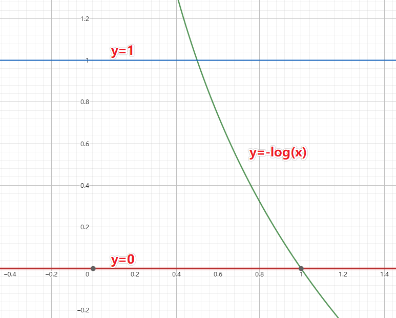
当真实标签 $y=1$ 时，我们希望模型预测的概率 $\hat{y}$ 尽可能接近 $1$，因为我们期望样本属于类别 $1$。此时，损失函数的表达式为:

$$ L = -\log{\hat{y}} $$

当真实标签$y=0$时，我们希望模型预测的概率 $\hat{y}$ 尽可能接近 $0$，因为我们期望样本属于类别 $0$。此时，损失函数的表达式为:

$$ L = -\log{(1- \hat{y})} $$

因此，综合考虑，我们可以将单个样本的损失函数表示为：

$$ L = -(y \cdot \log{\hat{y}} +(1-y) \cdot \log{(1- \hat{y})}) $$

其中，$y$ 表示真实标签，$\hat{y}$ 表示模型预测的标签。在二分类问题中，$y$ 只能取 0 或 1。

对于多个样本的情况，可以将每个样本的损失函数值相加或平均，得到总的损失函数值。例如，对于有$m$个样本的情况，可以使用以下公式计算总的交叉熵损失：

$$ J = - \frac{1}{m}\sum\_{i=1}^{m}(y^{(i)} \cdot \log{\hat{y}^{(i)}} + (1-y^{(i)}) \cdot \log{(1- \hat{y}^{(i)})}) $$

交叉熵损失函数的作用是通过最小化损失值来优化模型的参数，使模型的预测结果与真实标签更加接近。在训练过程中，模型会根据损失函数的反馈来调整参数，以提高预测的准确性。

示例

交叉熵损失函数通常用于分类问题中，其输入通常包括两个矩阵：一个是实际的标签（真实值），另一个是模型的预测值（概率分布）。这两个矩阵的形状一般是相同的，通常是 $(N, C)$，其中 $N$ 是样本数，$C$ 是类别数。

举个例子，假设我们有3个样本，每个样本可以属于3个类别之一。我们的真实标签和模型预测值如下：

真实标签（one-hot 编码）：

$$ y\_{true} = \begin{bmatrix} 1 & 0 & 0 \\ 0 & 1 & 0 \\ 0 & 0 & 1 \end{bmatrix} $$

模型预测值（概率分布）：

$$ y\_{pred} = \begin{bmatrix} 0.7 & 0.2 & 0.1 \\ 0.1 & 0.8 & 0.1 \\ 0.2 & 0.2 & 0.6 \end{bmatrix} $$

交叉熵损失函数的公式是：

$$ L = -\frac{1}{N} \sum*{i=1}^{N} \sum*{c=1}^{C} y*{i,c} \log{(\hat{y}*{i,c})} $$

其中 $y_{i,c}$ 是实际的标签，$\hat{y}_{i,c}$ 是预测的概率。

我们可以用Python代码来实现这个计算：

import numpy as np

# 真实标签 (one-hot 编码)
y_true = np.array([
    [1, 0, 0],
    [0, 1, 0],
    [0, 0, 1]
])

# 模型预测值 (概率分布)
y_pred = np.array([
    [0.7, 0.2, 0.1],
    [0.1, 0.8, 0.1],
    [0.2, 0.2, 0.6]
])

# 计算交叉熵损失
# 先对预测值取对数，然后逐元素乘以真实标签
log_preds = np.log(y_pred)
cross_entropy_loss = -np.sum(y_true * log_preds) / y_true.shape[0]

print("交叉熵损失:", cross_entropy_loss)

上述代码的执行结果是：

交叉熵损失: 0.3644204305930986

这说明了如何将真实标签和预测值矩阵传给交叉熵损失函数并计算损失值。注意，预测值矩阵中的每个元素必须是一个介于0和1之间的概率，并且每行的概率之和应该为1。

第三节 更新权重矩阵的过程

在机器学习中，权重矩阵 $W'$ 和损失函数 $L$ 的梯度 $\frac{\partial L}{\partial W'}$ 通常都是矩阵，而不是单一的数字。我们通过矩阵运算来更新权重，而不是逐元素进行标量计算。

具体来说，权重更新公式：

$$ W' = W' - \eta \cdot \frac{\partial L}{\partial W'} $$

是逐元素更新矩阵中的每一个元素。这些更新操作是基于每个元素的梯度和学习率 (\eta)。

下面举一个简单的例子，来演示如何进行这样的矩阵更新。

假设我们有一个非常简单的神经网络，只有一个权重矩阵 $W'$，其形状是 $2 \times 2$：

$$ W' = \begin{bmatrix} 0.1 & 0.2 \\ 0.3 & 0.4 \end{bmatrix} $$

假设损失函数 (L) 关于 (W’) 的梯度是：

$$ \frac{\partial L}{\partial W'} = \begin{bmatrix} 0.01 & 0.02 \\ 0.03 & 0.04 \end{bmatrix} $$

我们选择一个学习率 $\eta = 0.1$。

根据权重更新公式，我们计算新的权重矩阵 $W'$：

$$ W' = W' - \eta \cdot \frac{\partial L}{\partial W'} $$

让我们具体计算一下：

$$ \begin{aligned} W' &= \begin{bmatrix} 0.1 & 0.2 \\ 0.3 & 0.4 \end{bmatrix} - 0.1 \cdot \begin{bmatrix} 0.01 & 0.02 \\ 0.03 & 0.04 \end{bmatrix} \\ \\&= \begin{bmatrix} 0.1 - 0.1 \cdot 0.01 & 0.2 - 0.1 \cdot 0.02 \\ 0.3 - 0.1 \cdot 0.03 & 0.4 - 0.1 \cdot 0.04 \end{bmatrix} \\ \\&= \begin{bmatrix} 0.1 - 0.001 & 0.2 - 0.002 \\ 0.3 - 0.003 & 0.4 - 0.004 \end{bmatrix} \\ \\&= \begin{bmatrix} 0.099 & 0.198 \\ 0.297 & 0.396 \end{bmatrix} \end{aligned} $$

可以使用 Python 代码来进行上述计算：

import numpy as np

# 初始权重矩阵
W = np.array([
    [0.1, 0.2],
    [0.3, 0.4]
])

# 损失函数关于权重矩阵的梯度
dL_dW = np.array([
    [0.01, 0.02],
    [0.03, 0.04]
])

# 学习率
eta = 0.1

# 更新权重矩阵
W_updated = W - eta * dL_dW

print("更新后的权重矩阵:")
print(W_updated)

执行上述代码的结果会是：

更新后的权重矩阵:
[[0.099 0.198]
 [0.297 0.396]]

这展示了如何在矩阵形式下进行权重更新。通过这种方式，我们可以有效地处理神经网络中多个参数的更新，而不仅仅是单个数值的计算。

第四节 似然与对数似然

3.1 似然（Likelihood）

定义：似然是在已知观测数据的前提下，用来评估不同模型参数值的合理性或适合度的一种度量。与概率不同，似然是从观测数据的角度来评估模型参数，而不是从模型参数的角度来评估数据。

公式：假设我们有一个模型，其参数为$\theta$，观测数据为$X$。似然函数$L(\theta|X)$定义为：

$$ L(\theta | X) = P(X | \theta) $$

这表示在参数$\theta$给定的情况下，观测到数据$X$的概率。

3.2 对数似然（Log-Likelihood）

定义：对数似然是似然的对数变换，用于简化计算和分析。对数似然保留了似然函数的性质，但由于对数的单调递增性，最大化对数似然与最大化似然是等价的。

公式：对于观测数据$X$和参数$\theta$，对数似然函数$\ell(\theta|X)$定义为：

$$ \ell(\theta | X) = \log L(\theta | X) $$

对于独立同分布的数据$X = (x_1, x_2, \ldots, x_n)$，似然函数为：

$$ L(\theta | X) = \prod\_{i=1}^n P(x_i | \theta) $$

对应的对数似然为：

$$ \begin{aligned} \ell(\theta | X) &= \log \left( \prod*{i=1}^n P(x_i | \theta) \right) \\&= \sum*{i=1}^n \log P(x_i | \theta) \end{aligned} $$

3.3 具体例子：二项分布模型

假设我们有一个二项分布模型来描述掷硬币的过程，参数 $\theta$ 表示正面出现的概率。我们进行了10次掷硬币实验，结果为6次正面和4次反面。观测数据$X$为6个正面和4个反面。

1. 似然函数

   似然函数表示在参数$\theta$下，观测到6次正面和4次反面的概率：

   $$ L(\theta | X) = \theta^6 (1 - \theta)^4 $$

2. 对数似然函数

   对数似然函数表示为：

$$ \begin{aligned} \ell(\theta | X) &= \log L(\theta | X) \\&= \log(\theta^6 (1 - \theta)^4) \\&= 6 \log \theta + 4 \log (1 - \theta) \end{aligned} $$

计算具体值:

为了找到最大似然估计，我们需要对对数似然函数求导并找到其最大值。

1. 对数似然函数为：

$$ \ell(\theta | X) = 6 \log \theta + 4 \log (1 - \theta) $$

2. 对数似然函数的导数

   为了找到最大似然估计，我们对对数似然函数求导，并令导数等于0：

$$ \frac{d}{d\theta} \ell(\theta | X) = \frac{6}{\theta} - \frac{4}{1 - \theta} $$

设置导数等于0：

$$ \frac{6}{\theta} - \frac{4}{1 - \theta} = 0 $$

解这个方程：

$$ \frac{6}{\theta} = \frac{4}{1 - \theta} $$

交叉相乘得到：

$$ 6(1 - \theta) = 4\theta $$

展开并整理：

$$ 6 - 6 \cdot \theta = 4 \cdot \theta $$ $$ 6 = 10 \cdot \theta $$ $$ \theta = \frac{6}{10} = 0.6 $$

3. 计算对数似然值

   在$\theta = 0.6$时，对数似然函数的值：

$$ \begin{aligned} \ell(0.6 | X) &= 6 \log 0.6 + 4 \log (1 - 0.6) \\&= 6 \times (-0.5108) + 4 \times (-0.9163) \\&= -3.0648 + (-3.6652) \\&= -6.73 \end{aligned} $$

4. 计算似然值

   在$\theta = 0.6$时，观测到6次正面和4次反面的概率：

$$ \begin{aligned} L(0.6 | X) &= 0.6^6 \times 0.4^4 \\&= 0.046656 \times 0.0256 \\&\approx 0.001194 \end{aligned} $$

似然衡量的是在给定参数值下观测到特定数据的概率，对数似然是其对数变换，用于简化计算。通过最大似然估计，我们找到参数$\theta = 0.6$，使得观测数据6次正面和4次反面的对数似然最大。对数似然值为$-6.73$，对应的似然值为$0.001194$。通过这种方法，我们可以确定模型参数，并评估其在给定数据下的合理性。

第五节 示例代码

https://github.com/weberrr/pytorch_word2vec